Abstract
AbstractWe report a deep learning-enabled field-portable and cost-effective imaging flow cytometer that automatically captures phase-contrast color images of the contents of a continuously flowing water sample at a throughput of 100 mL/h. The device is based on partially coherent lens-free holographic microscopy and acquires the diffraction patterns of flowing micro-objects inside a microfluidic channel. These holographic diffraction patterns are reconstructed in real time using a deep learning-based phase-recovery and image-reconstruction method to produce a color image of each micro-object without the use of external labeling. Motion blur is eliminated by simultaneously illuminating the sample with red, green, and blue light-emitting diodes that are pulsed. Operated by a laptop computer, this portable device measures 15.5 cm × 15 cm × 12.5 cm, weighs 1 kg, and compared to standard imaging flow cytometers, it provides extreme reductions of cost, size and weight while also providing a high volumetric throughput over a large object size range. We demonstrated the capabilities of this device by measuring ocean samples at the Los Angeles coastline and obtaining images of its micro- and nanoplankton composition. Furthermore, we measured the concentration of a potentially toxic alga (Pseudo-nitzschia) in six public beaches in Los Angeles and achieved good agreement with measurements conducted by the California Department of Public Health. The cost-effectiveness, compactness, and simplicity of this computational platform might lead to the creation of a network of imaging flow cytometers for large-scale and continuous monitoring of the ocean microbiome, including its plankton composition.
🔬 Techniques
✨ Fluorophores
🏭 Microscope Brands
🧪 Reagent Suppliers
🏛️ Research Organizations (ROR)
Affiliated research institutions:
📋 Methods
Optical system
Our imaging flow cytometer uses a color image sensor with a pixel size of 1.4 µm (Basler aca4600-10uc). The housing of the camera is removed, and the circuit is rearranged to allow the sample holder to be placed in direct contact with the protective cover glass of the image sensor (see Fig. 1 ). Illumination of the holographic microscope is provided by using the red, green, and blue emitters from a light-emitting diode (LED) (Ledengin LZ4-04MDPB). The spatial and temporal coherence of the emitted light from the LEDs is increased to achieve the maximum resolution allowed by the sensor pixel size. The spatial coherence is adjusted by using a convex mirror (Edmund Optics #64-061) to increase the light path. The LED light is also spectrally filtered by two triple-bandpass optical filters (Edmund Optics #87–246, Chroma Inc. 69015m) to increase the temporal coherence of the illumination. The placement of the optical components is designed to tune the bandpass of the spectral filter angle to better match the emission maximum of the LEDs. Increasing the spatial and temporal coherence of the LEDs also decreases the intensity reaching the image sensor. In addition, the short exposure time required to avoid the motion blur when imaging objects in a fast flow makes it necessary for our configuration to utilize a linear sensor gain of 2. The additional noise generated from the gain is sufficiently low as to not interfere with the image-reconstruction process.
Microfluidic channel and flow design
A microfluidic channel (Ibidi µ-Slide I) with an internal height of 0.8 mm is placed on the top of the image sensor, secured using a three-dimensional (3D)-printed holder, and connected to a peristaltic pump (Instech p625). The size of the active area of the image sensor is slightly smaller than the width of the channel (4.6 mm vs. 5 mm), and the channel is positioned so that the sensor measures the center of the liquid flow. We calculated the flow profile inside the channel (see Fig. 6 ) by solving the Navier–Stokes equation for noncompressible liquids assuming a nonslip boundary condition. The results show that the image sensor measures ~98% of the total volume passing through the microfluidic channel. The flow profile is a two-dimensional paraboloid, with the maximum flow speed located at the center of the microfluidic channel and measuring approximately 1.66 times higher than the mean velocity of the liquid (see Fig. 6 ). To acquire sharp, in-focus images of the objects in the continuously flowing liquid, we operate the image sensor in the global reset release mode and illuminated the sample by flash pulses, where the length of an illuminating pulse is adjusted to not allow an object traveling at the maximum speed inside the channel to shift by more than the width of a single sensor pixel. For a flowrate of 100 mL/h, this corresponds to a pulse length of 120 µs. Pulsed illumination, power, and control circuit Because shortening the illumination time also constrains the available photon budget, we maximize the brightness of our LEDs by operating them at currents ranging from 2.2 to 5 A depending on their color. The currents are set for each LED emitter to create similar brightness levels at our image sensor, ensuring that we adequately light the sample at each color, a requirement for obtaining color images. The green LED spectrum is inherently wider than the red and blue counterparts, and thus the spectral filters will reduce its intensity the most. Therefore, we operate the green LED at the experimentally determined maximum possible current of 5 A. The red and blue LEDs require a current of ~2.2 A to match the intensity of the green LED on the image sensor to correct the white balance. We designed a circuit to control the necessary components of the device. The circuit is powered by either a 5-V wall-mounted power supply or a cellphone charger battery pack. The circuit fulfills four major roles: providing power to the peristaltic pump, charging the capacitors for providing power to the LEDs, synchronizing the LEDs to the camera and creating stable, short, high current pulses, and, finally, providing an interface for remote control by a laptop using an Inter-Integrated-Circuit (i2c) interface for setting various parameters. The peristaltic pump is powered by a high-efficiency step-up DC-DC converter at 16 V ( TPS61086 , Texas instruments), and its speed is controlled by a potentiometer via i2c components (TPL0401B, Texas Instruments). The charge for the high-current pulses is stored in three 0.1-F capacitors, which are charged using a capacitor charger controller (LT3750, Linear Technologies) to 12 V. The capacitor charge is initiated by the image sensor flash window trigger signal, which is active during the frame capture, and its length can be controlled by the camera software driver. The charger controller acquires an “on” state and keeps charging the capacitors until the preset voltage level of 12 V is reached. During the short illumination pulses, the voltage on the capacitors decreases only slightly, and they are immediately recharged as each frame capture resets the charge cycle, thereby allowing continuous operation. The LEDs are synchronized and their constant-current operation is ensured by a triple-output LED driver controller (LT3797, Linear Technologies). The controller uses the same flash window signal from the image sensor to turn on the LEDs for the exposure duration set by the software. The current of each LED is controlled between 0 and 12.5 A using digital i2c potentiometers (TPL0401A, Texas Instruments) and is kept constant for the subsequent pulses by the circuit, thus maintaining the same illumination intensity for each holographic frame. During startup, it takes ~3–4 frames for the circuit to stabilize at a constant light level. To avoid having multiple devices with the same address on the i2c line, we included an address translator (LTC4317, Linear Technologies) to interface with the potentiometers controlling the red and blue LEDs. To control the circuit, the laptop communicates with an Arduino microcontroller (TinyDuino from Tinycircuits), which is used as an interface for i2c communications only. During the initial startup, the circuit consumes ~1 A for the first ~8 s until the capacitors are fully charged. During its operation, the circuit consumes, on average, ~370 mA with a pump speed setting of 100 mL/h and a frame rate of 3 frames per second. This yields an average power consumption of less than 2 W. In addition, the image sensor’s typical power consumption is ~2.8 W according to the manufacturer’s data.
Show full methods section
Optical system
Our imaging flow cytometer uses a color image sensor with a pixel size of 1.4 µm (Basler aca4600-10uc). The housing of the camera is removed, and the circuit is rearranged to allow the sample holder to be placed in direct contact with the protective cover glass of the image sensor (see Fig. 1 ). Illumination of the holographic microscope is provided by using the red, green, and blue emitters from a light-emitting diode (LED) (Ledengin LZ4-04MDPB). The spatial and temporal coherence of the emitted light from the LEDs is increased to achieve the maximum resolution allowed by the sensor pixel size. The spatial coherence is adjusted by using a convex mirror (Edmund Optics #64-061) to increase the light path. The LED light is also spectrally filtered by two triple-bandpass optical filters (Edmund Optics #87–246, Chroma Inc. 69015m) to increase the temporal coherence of the illumination. The placement of the optical components is designed to tune the bandpass of the spectral filter angle to better match the emission maximum of the LEDs. Increasing the spatial and temporal coherence of the LEDs also decreases the intensity reaching the image sensor. In addition, the short exposure time required to avoid the motion blur when imaging objects in a fast flow makes it necessary for our configuration to utilize a linear sensor gain of 2. The additional noise generated from the gain is sufficiently low as to not interfere with the image-reconstruction process.
Microfluidic channel and flow design
A microfluidic channel (Ibidi µ-Slide I) with an internal height of 0.8 mm is placed on the top of the image sensor, secured using a three-dimensional (3D)-printed holder, and connected to a peristaltic pump (Instech p625). The size of the active area of the image sensor is slightly smaller than the width of the channel (4.6 mm vs. 5 mm), and the channel is positioned so that the sensor measures the center of the liquid flow. We calculated the flow profile inside the channel (see Fig. 6 ) by solving the Navier–Stokes equation for noncompressible liquids assuming a nonslip boundary condition. The results show that the image sensor measures ~98% of the total volume passing through the microfluidic channel. The flow profile is a two-dimensional paraboloid, with the maximum flow speed located at the center of the microfluidic channel and measuring approximately 1.66 times higher than the mean velocity of the liquid (see Fig. 6 ). To acquire sharp, in-focus images of the objects in the continuously flowing liquid, we operate the image sensor in the global reset release mode and illuminated the sample by flash pulses, where the length of an illuminating pulse is adjusted to not allow an object traveling at the maximum speed inside the channel to shift by more than the width of a single sensor pixel. For a flowrate of 100 mL/h, this corresponds to a pulse length of 120 µs. Pulsed illumination, power, and control circuit Because shortening the illumination time also constrains the available photon budget, we maximize the brightness of our LEDs by operating them at currents ranging from 2.2 to 5 A depending on their color. The currents are set for each LED emitter to create similar brightness levels at our image sensor, ensuring that we adequately light the sample at each color, a requirement for obtaining color images. The green LED spectrum is inherently wider than the red and blue counterparts, and thus the spectral filters will reduce its intensity the most. Therefore, we operate the green LED at the experimentally determined maximum possible current of 5 A. The red and blue LEDs require a current of ~2.2 A to match the intensity of the green LED on the image sensor to correct the white balance. We designed a circuit to control the necessary components of the device. The circuit is powered by either a 5-V wall-mounted power supply or a cellphone charger battery pack. The circuit fulfills four major roles: providing power to the peristaltic pump, charging the capacitors for providing power to the LEDs, synchronizing the LEDs to the camera and creating stable, short, high current pulses, and, finally, providing an interface for remote control by a laptop using an Inter-Integrated-Circuit (i2c) interface for setting various parameters. The peristaltic pump is powered by a high-efficiency step-up DC-DC converter at 16 V ( TPS61086 , Texas instruments), and its speed is controlled by a potentiometer via i2c components (TPL0401B, Texas Instruments). The charge for the high-current pulses is stored in three 0.1-F capacitors, which are charged using a capacitor charger controller (LT3750, Linear Technologies) to 12 V. The capacitor charge is initiated by the image sensor flash window trigger signal, which is active during the frame capture, and its length can be controlled by the camera software driver. The charger controller acquires an “on” state and keeps charging the capacitors until the preset voltage level of 12 V is reached. During the short illumination pulses, the voltage on the capacitors decreases only slightly, and they are immediately recharged as each frame capture resets the charge cycle, thereby allowing continuous operation. The LEDs are synchronized and their constant-current operation is ensured by a triple-output LED driver controller (LT3797, Linear Technologies). The controller uses the same flash window signal from the image sensor to turn on the LEDs for the exposure duration set by the software. The current of each LED is controlled between 0 and 12.5 A using digital i2c potentiometers (TPL0401A, Texas Instruments) and is kept constant for the subsequent pulses by the circuit, thus maintaining the same illumination intensity for each holographic frame. During startup, it takes ~3–4 frames for the circuit to stabilize at a constant light level. To avoid having multiple devices with the same address on the i2c line, we included an address translator (LTC4317, Linear Technologies) to interface with the potentiometers controlling the red and blue LEDs. To control the circuit, the laptop communicates with an Arduino microcontroller (TinyDuino from Tinycircuits), which is used as an interface for i2c communications only. During the initial startup, the circuit consumes ~1 A for the first ~8 s until the capacitors are fully charged. During its operation, the circuit consumes, on average, ~370 mA with a pump speed setting of 100 mL/h and a frame rate of 3 frames per second. This yields an average power consumption of less than 2 W. In addition, the image sensor’s typical power consumption is ~2.8 W according to the manufacturer’s data.
Object detection and deep learning-based hologram reconstruction
For automatic detection and holographic reconstruction of the target objects found in the continuously flowing water sample (see Fig. 7 ), the static objects found in the raw full FOV image (e.g., dust particles in the flow channel) need to be eliminated first. This is achieved by calculating a time-averaged image of the preceding ~20 images containing only the static objects and subtracting it from the present raw hologram. To ensure appropriate reconstruction quality, the mean of this subtracted image is added back uniformly to the current frame. This yields a background-subtracted full FOV image in which only the holograms of the objects newly introduced by the flow are present. These objects are automatically detected and segmented from the full FOV for individual processing (see Supplementary Figure S2 ). The full FOV background-subtracted hologram is first Gaussian-filtered and converted into a binary image by hard-thresholding with its statistical values (mean + 1.5 × standard deviation), which isolates the peaks of the holographic signatures created by the objects included in the FOV. The binary contours with an area of a few pixels are removed to reduce misdetection events due to sensor noise. A closing operation is performed in the generated binary image to create a continuous patch for each object. The resulting binary contours represent the shapes and locations of the objects appearing in the FOV, and their morphological information is used to filter each contour by certain desired criteria (e.g., major axis). The center coordinate of the filtered contour is used to segment its corresponding hologram. We should emphasize that not only is it feasible to extract all objects in the FOV but it is also possible to prioritize the segmentation of the objects of interest for a specific goal by our approach. Thus, we can better utilize the computational resources of the laptop and maintain real-time processing for denser samples. After segmentation, the Bayer-patterned holograms are separated into three mono-color (i.e., red, green, and blue) holograms corresponding to the illumination wavelengths. To fully utilize the spatial resolution of the optical system, the orientation of the Bayer-patterned green pixels is rotated by 45° to regularize their sampling grid 40 . Concurrently, the red and blue mono-color holograms are upsampled by a factor of two, and a 45° rotation is applied to these upsampled holograms. These processes are jointly called “Resampling” in Fig. 7 . Holographic autofocusing using the Tamura coefficient of the complex gradient 41 , 42 is performed for each segmented object using only a single mono-color hologram to accurately estimate the distance of the respective object from the image sensor plane. At this point, we have 3D localized each object within the flow (per FOV). The coordinates of each detected object are then used in conjunction with the estimated flow profile from our calculations, and the location of each object is predicted at the next frame. If an object is found at the predicted coordinates, it is flagged to be removed from the total count and processing workflow to avoid reconstructing and counting the same object multiple times. At this point, the image preprocessing step (shown in cyan in Fig. 7 ) is complete. Fig. 7 The algorithm used for object segmentation and deep learning-based hologram reconstruction in our field-portable imaging flow cytometer is illustrated. The phase-recovered intensity and phase images in red, green, and blue channels are fused to generate a final phase-contrast image per object (shown within the dashed black frame on the right) The next step is the high-resolution color reconstruction (shown in pink in Fig. 7 ). We maximize the resolution of the reconstruction by further upsampling the holograms by a factor of four. Each color channel is then propagated to the obtained reconstruction distance by an angular spectrum-based wave-propagation algorithm 26 and thus brought into focus. The slight incidence angle difference between the red, green, and blue emitters is corrected by modifying the propagation kernel accordingly 43 . To evaluate the resolution of the imaging flow cytometer system for the objects located inside our microfluidic channel, we replaced the flow channel with a 1951 Air Force test chart (see Supplementary Figure S3 ). Due to the partially coherent nature of our illumination, the resolution depends on the object–sensor distance; thus, we measured it by placing the test chart at various heights above the sensor. The width of the smallest resolved line varied between 1.55 µm and 1.95 µm depending on the height of the object, with 1.55 µm corresponding to the smallest resolvable feature for most flowing objects imaged by the imaging flow cytometer during its regular operation. These raw reconstructions, however, are contaminated by self-interference and twin-image noise, which are characteristic of in-line digital holographic imaging systems due to the loss of the phase information of the hologram at the sensor plane. To achieve accurate image reconstruction without these artifacts, a deep learning-based digital holographic phase recovery method 38 , 44 was employed using a convolutional neural network (see Fig. 7 and Supplementary Figure S4 ) pretrained with various phase-recovered reconstructions of water-borne micro-objects captured with our imaging flow cytometer. This method enables automated and accurate acquisition of the spectral morphology of an object without sacrificing the high-throughput operation of the holographic imaging cytometer, which otherwise would be very challenging as other existing phase-recovery methods require static repetitive measurements 43 , 45 – 48 and/or time-consuming iterative calculations 43 , 45 – 50 , which would not work for flowing objects. For the visualization of transparent objects, such as plankton, we computed the color phase-contrast image based on the complex-valued reconstructions of the red, green, and blue channels, which assist in accurately resolving the fine features and internal structures of various water-borne microorganisms with high color contrast (see, e.g., Figs. 2 , 3 , and 7 ). The phase-contrast image was synthesized by (1) estimating the background field from the mean amplitude and phase of the refocused complex field, (2) calculating the object field by subtracting the background field from the refocused field, (3) shifting the phase of the background field by π /2, (4) adding the phase-shifted background field to the object field, and (5) taking the magnitude of the recalculated total field. Graphical user interface We developed a GUI to operate the device. Through this GUI, all relevant measurement parameters can be specified, such as the liquid flow speed, the driving currents, the incidence angles for the red, green, and blue LEDs, the flash pulse duration, and the camera sensor gain. The GUI gives a real-time, full FOV reconstructed image at the center of the channel, thus allowing visual inspection during flow with and without background subtraction, and displays the total number of detected objects in the current frame. The GUI is also capable of visualizing up to 12 segmented, autofocused, and reconstructed objects in real time. The user can specify whether to digitally save any combination of the raw, background-subtracted holograms or reconstructed images. The GUI can also be run in demo mode to analyze previously captured image datasets without the presence of the imaging flow cytometer.
Sample preparation and analysis
We followed the sampling protocol recommended by CDPH (USA) to obtain our ocean samples. We used a plankton net with a diameter of 25 cm and a mesh size of 20 µm and performed vertical tows with a total length of 15 m (5 × 3 m) from the end of the pier at each sampling location where a pier was present (Malibu, Santa Monica, Venice, Manhattan, and Redondo; California, USA). There was no pier at Point Dume; thus, we performed a horizontal tow from the shoreline. The plankton net condensed the micro- and nanoplankton found in the ocean into a sample volume of ~250 mL; i.e., in our case, a condensation ratio of ~3000×. We extracted 1 mL of the condensed sample, rediluted it with 50 mL of filtered ocean water, and imaged its contents using our imaging flow cytometer. The remaining samples were sent to CDPH for subsequent analysis (used for comparison purposes). During our field tests, we used the same plankton net but only performed one vertical tow from a depth of 1.5 m at each measurement. A 1-mL aliquot of the obtained sample was rediluted with 20 mL of filtered ocean water. To conserve the battery power of the controlling laptop, ~12 mL of this sample was imaged on-site. The imaging flow cytometer automatically detected and saved the reconstructed images of all detected plankton and provided the user real-time feedback on the total plankton count detected. Specific counting of Pseudo-nitzschia was performed manually by scanning through the dataset of the saved images and visually identifying Pseudo-nitzschia .
Electronic supplementary material Supplementary Information
Electronic supplementary material Supplementary information is available for this paper at 10.1038/s41377-018-0067-0.
📊 Figures
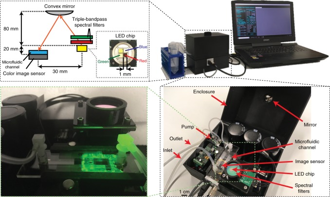
Fig. 1
Photos and schematic of the imaging flow cytometer device.
The water sample is constantly pumped through the microfluidic channel at a rate of 100u2009mL/h during imaging. The illumination is emitted simultaneously from red, green, and blue LEDs in 120-u00b5s...
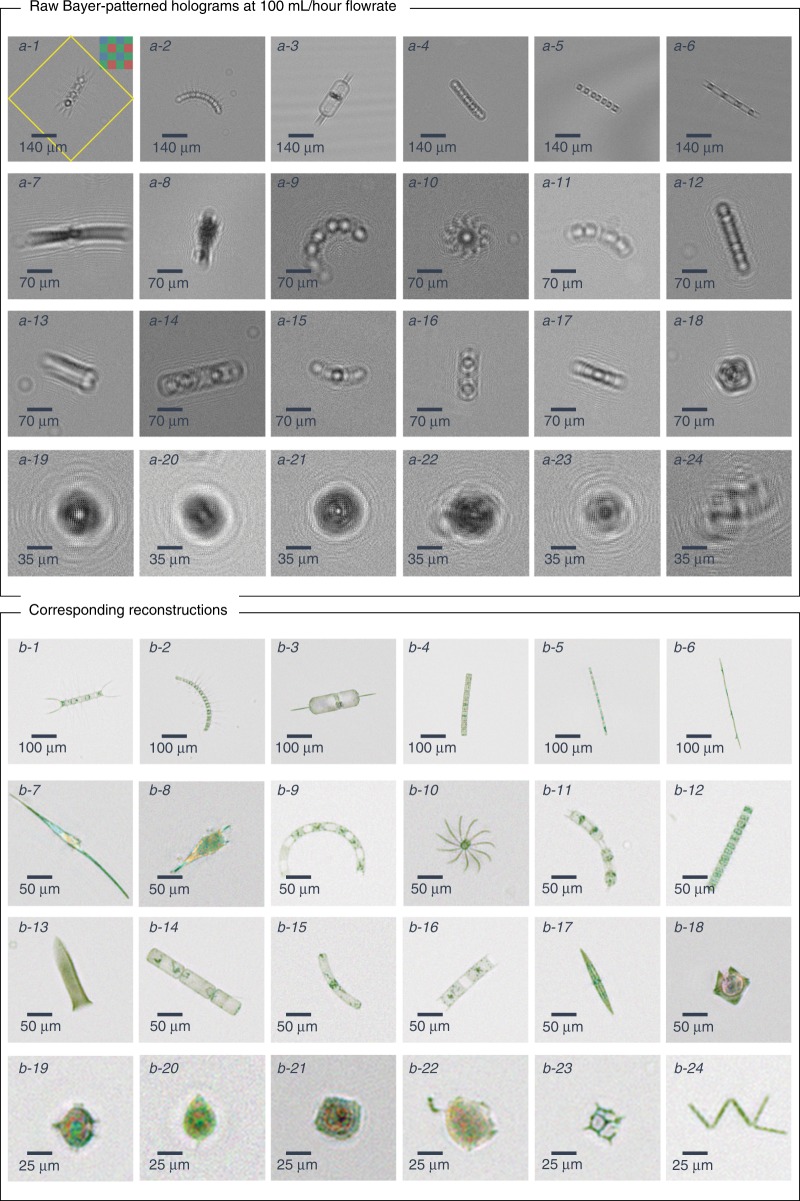
Fig. 2
The image quality of the flow cytometer allows the identification of plankton.
Examples of various ocean planktons detected by our imaging flow cytometer at the Los Angeles coastline, represented by their a raw holograms and b phase-contrast reconstructions following phase recov...
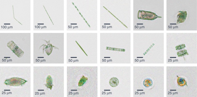
Fig. 3
Reconstructed images of various phytoplankton and zooplankton.
Phase-contrast color images depicting the plankton found near the Los Angeles coastline and imaged by our flow cytometer at a flowrate of 100u2009mL/h
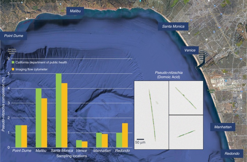
Fig. 4
Prevalence of Pseudo-nitzschia in the ocean along the Los Angeles coastline on January 31, 2018.
Samples were collected according to California Department of Public Health (CDPH) protocols. A portion of each sample was analyzed by the imaging flow cytometer system, and the remainder was sent to C...
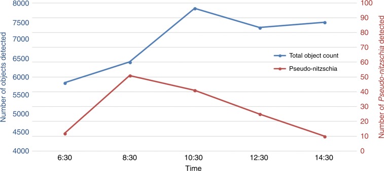
Fig. 5
Field test results from a series of measurements at Redondo Beach on April 17, 2018.
We sampled the top 1.5u2009m of the ocean every 2u2009h and measured on-site the variation in the plankton concentration over time. The measurements started after sunrise (6:21 am), and each sample wa...
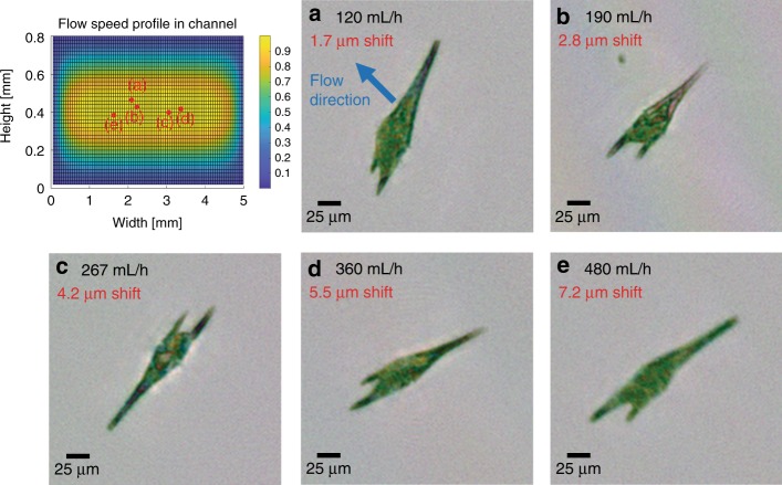
Fig. 6
Effect of increasing the liquid flow speed in the system on the image quality.
The relative flow speed profile inside the rectangular channel cross-section is depicted in the top left (see the Methods section). The measurements were made on an ocean sample containing a high conc...
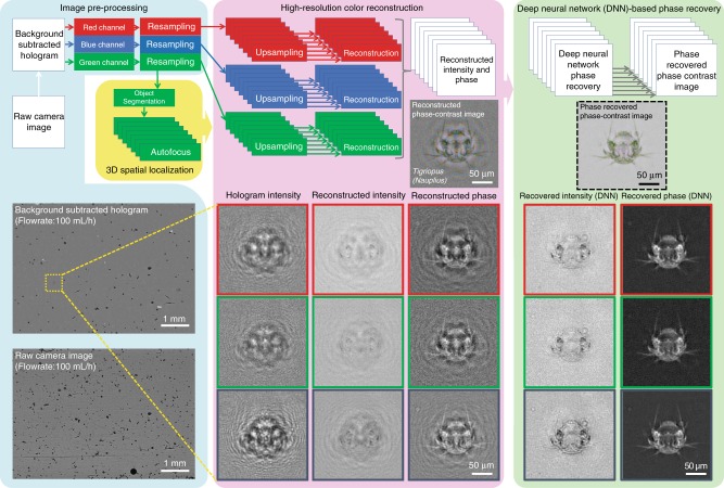
Fig. 7
The algorithm used for object segmentation and deep learning-based hologram reconstruction in our field-portable imaging flow cytometer is illustrated.
The phase-recovered intensity and phase images in red, green, and blue channels are fused to generate a final phase-contrast image per object (shown within the dashed black frame on the right)
Figure images are served from the NIH/NLM PubMed Central Open Access Subset or Europe PMC; copyright remains with the publishers and authors.
💬 Discussion
0 commentsNo comments yet. Be the first to start a discussion!
Leave a Comment