Abstract
Recent studies have supported the relation between mitochondrial functions and degenerative disorders related to ageing, such as Alzheimer's and Parkinson's diseases. Since these studies have exposed the need for detailed and high-resolution analysis of physical alterations in mitochondria, it is necessary to be able to perform segmentation and 3D reconstruction of mitochondria. However, due to the variety of mitochondrial structures, automated mitochondria segmentation and reconstruction in electron microscopy (EM) images have proven to be a difficult and challenging task. This paper puts forward an effective and automated pipeline based on deep learning to realize mitochondria segmentation in different EM images. The proposed pipeline consists of three parts: (1) utilizing image registration and histogram equalization as image pre-processing steps to maintain the consistency of the dataset; (2) proposing an effective approach for 3D mitochondria segmentation based on a volumetric, residual convolutional and deeply supervised network; and (3) employing a 3D connection method to obtain the relationship of mitochondria and displaying the 3D reconstruction results. To our knowledge, we are the first researchers to utilize a 3D fully residual convolutional network with a deeply supervised strategy to improve the accuracy of mitochondria segmentation. The experimental results on anisotropic and isotropic EM volumes demonstrate the effectiveness of our method, and the Jaccard index of our segmentation (91.8% in anisotropy, 90.0% in isotropy) and F1 score of detection (92.2% in anisotropy, 90.9% in isotropy) suggest that our approach achieved state-of-the-art results. Our fully automated pipeline contributes to the development of neuroscience by providing neurologists with a rapid approach for obtaining rich mitochondria statistics and helping them elucidate the mechanism and function of mitochondria.
🔬 Techniques
🧪 Sample Preparation
🏭 Microscope Brands
💻 Software Details
🏛️ Research Organizations (ROR)
Affiliated research institutions:
📋 Methods
In this section, we provide a detailed description of the datasets and pipeline of our proposed method. The datasets consist of anisotropic and isotropic EM volumes, which are widely used in the evaluation of mitochondria segmentation. As illustrated in Figure 1 , the proposed automated mitochondria segmentation method for EM datasets can be divided into three parts: image pre-processing, mitochondria segmentation with the proposed 3D convolutional network and 3D visualization. All procedures were approved by the Animal Committee of the Institute of Neuroscience, Chinese Academy of Sciences (CAS). Figure 1 The pipeline of our proposed method. (Left to Right) Image pre-processing with registration and histogram equalization; mitochondria segmentation with the proposed 3D residual FCN; 3D connection and visualization in ImageJ. 2.1.
Image datasets
The details of each dataset are summarized in Table 1 and Figure 2 . The public FIB-SEM dataset 2 from a rat hippocampus was acquired by Graham Knott and Marco Cantoni at École Polytechnique Fédérale de Lausanne (EPFL) (Lucchi et al., 2013 ). In this dataset, the mitochondria were annotated in two volumes: training volume and testing volume. The training dataset consists of a stack of 165 slices from the FIB-SEM dataset, which measures approximately 3.84 × 5.12 × 0.83 μm 3 with a resolution of 5 × 5 × 5 nm 3 per voxel. The testing dataset with 165 slices was obtained from a different part of the same specimens. Table 1 Illustration of two datasets. Dataset EM Voxel size ( nm 3 ) Train size Test size Cortex ATUM-SEM 2 × 2 × 50 8,624 × 8,416 × 20 8,624 × 8,416 × 11 Hippocampus FIB-SEM 5 × 5 × 5 1,024 × 768 × 165 1,024 × 768 × 165 Figure 2 Illustration of the datasets. (A) Isotropic image from mouse hippocampus obtained by FIB-SEM; (B) Ground truth of the FIB-SEM image; (C) Anisotropic image from rat cortex acquired by ATUM-SEM; (D) Ground truth of the ATUM-SEM image. Scale bar: 500 nm. In the ATUM-SEM dataset from a mouse cortex, which was acquired by the Institute of Neuroscience, CAS, 31 sections with thicknesses of approximately 50 nm were cut automatically (Yang et al., 2016 ). Next, these sections were imaged through a Zeiss Supra55 microscope at the Institute of Automation, CAS, where the pixel size was set at 2 nm and the dwell time was set at 2 μs. The ground truths were annotated by neuroanatomists using ImageJ (Schmid et al., 2010 ) with the TrakEm2 plug-in (Cardona et al., 2012 ). Note that the production of such a ground truth database required a great amount of human effort, which served to justify that automated segmentation is liable to accelerate neuroscience analyses. 2.2. Pre-processing In this subsection, we presented the pre-processing method consisting of image registration and histogram equalization. The details are as follows. As mentioned above, the data imaged with the ATUM-SEM method were unregistered. The image registration method adopted (Li et al., 2017b ) for serial sections of biological tissue was divided into three parts: (1) searching for correspondences between adjacent sections; (2) displacement calculations for the identified correspondences; and (3) warping the image tiles based on the new position of these correspondences. For correspondence searching, we adopted the SIFT-flow algorithm (Liu et al., 2008 ) to search for correspondences between adjacent sections by extracting equally distributed grid points from the well-aligned adjacent sections. For the displacement calculation, the positions of the identified correspondences were adjusted throughout all sections by minimizing a target energy function, which consisted of a data term, a small displacement term, and a smoothness term. The data term keeps pairs of correspondences at the same positions in the x-y plane after displacement. The small displacement term constrains the correspondence displacements to minimize image deformation. The smoothness term constrains the displacement of the neighboring correspondences. For image warping, we used the moving least squares (MLS) method (Schaefer et al., 2006 ) to warp each section with the obtained positions. The deformation results produced by MLS are globally smooth to retain the shape of biological specimens. This image registration method not only reflects the discontinuity around wrinkle areas but also retains the smoothness in other regions, which provides a stable foundation for follow-up works. In addition, many factors, such as differences in slice thickness, polluted or uneven surfaces and an unstable electron beam, will produce an uneven grayscale between images. It is hard to maintain the acquired images with consistent pixel distributions during the imaging process. Occasionally, some images are much brighter than others, and these differences will inevitably increase the complexity of the images and make segmentation more challenging. To this end, histogram equalization was adopted to weaken the noise and enhance the contrast of raw images, which reduced the complexity of the images and improved the segmentation performance. 2.3. The proposed mitochondria segmentation network In this work, we combined the residual block with variant 3D U-Net to extend and deepen the network. There are three advantages to our proposed architecture: (1) the 3D convolution network is capable of exploiting the 3D spatial information from volumetric EM data, (2) the variant U-Net structure and residual convolution module could better extract features, and (3) injected auxiliary classifier layers could help avoid the problem of vanishing gradients. Figure 3 is a pictorial illustration of the proposed network. The components, such as the convolutional layers of the network, are implemented in a 3D manner; hence, the network could effectively extract 3D information from serial EM data. Additionally, the proposed network is a fully convolutional architecture and thus is capable of taking arbitrary-sized 3D data as input and producing corresponding size outputs, which is suitable for dealing with a large-scale serial EM dataset. Figure 3 The architecture of the proposed network. Blue blocks denote feature maps, and numbers imply the channel of feature maps in each layer. The red arrow represents the residual block, which consists of two 3D convolutional layers with a kernel size of 3 × 3 × 3 and a residual shortcut connection. As a variant of the U-Net, this network consists of a contracting path and an expansive path. The contracting path contains 13 convolutional layers, and the expansive path contains 15 convolutional layers; thus, the whole network is not entirely symmetric. Specifically, each path could be divided into different stages that operate in different receptive fields, and we adopted a 3D residual module to extract the features in each stage. The 3D residual module consists of two convolutional layers with a kernel size of 3 × 3 × 3 and a residual shortcut connection, each of which was followed by batch normalization (BN) and exponential linear unit (ELU) nonlinearity (to mitigate the internal covariate shift). Zero padding was used to preserve the size of the input feature maps. As confirmed by our empirical experiments, this residual architecture increased the number of ensemble sub-networks and was beneficial for feature extraction. In contrast to previous methods (Milletari et al., 2016 ; Lee et al., 2017 ), our residual block contains only two 3D convolutional layers, which maintains the effectiveness and needs fewer parameters. Given anisotropic ATUM-SEM images with a resolution of 2 × 2 × 50 nm 3 , the widely used max-pooling and upsampling layers (with a stride of 2 × 2 × 2) might lower the resolution of volumes in the z-dimension and reduce the accuracy of predictions. Therefore, we chose the max-pooling and upsampling layers with a stride 2 × 2 × 1 to deal with anisotropy images, which minimized the inferior information loss along the z-dimension. In the following, several summation-based skip connections were utilized to incorporate global information from higher layers and local cues from lower layers. Compared to concatenation-based skip connections, summation-based skip connections fused multilevel contextual information more thoroughly and helped handle the vanishing gradient problem. To further solve the problem of vanishing gradients, we injected auxiliary classifier layers into the hidden layers to train the network. The details are discussed in section 2.4. 2.4.
Show full methods section
In this section, we provide a detailed description of the datasets and pipeline of our proposed method. The datasets consist of anisotropic and isotropic EM volumes, which are widely used in the evaluation of mitochondria segmentation. As illustrated in Figure 1 , the proposed automated mitochondria segmentation method for EM datasets can be divided into three parts: image pre-processing, mitochondria segmentation with the proposed 3D convolutional network and 3D visualization. All procedures were approved by the Animal Committee of the Institute of Neuroscience, Chinese Academy of Sciences (CAS). Figure 1 The pipeline of our proposed method. (Left to Right) Image pre-processing with registration and histogram equalization; mitochondria segmentation with the proposed 3D residual FCN; 3D connection and visualization in ImageJ. 2.1.
Image datasets
The details of each dataset are summarized in Table 1 and Figure 2 . The public FIB-SEM dataset 2 from a rat hippocampus was acquired by Graham Knott and Marco Cantoni at École Polytechnique Fédérale de Lausanne (EPFL) (Lucchi et al., 2013 ). In this dataset, the mitochondria were annotated in two volumes: training volume and testing volume. The training dataset consists of a stack of 165 slices from the FIB-SEM dataset, which measures approximately 3.84 × 5.12 × 0.83 μm 3 with a resolution of 5 × 5 × 5 nm 3 per voxel. The testing dataset with 165 slices was obtained from a different part of the same specimens. Table 1 Illustration of two datasets. Dataset EM Voxel size ( nm 3 ) Train size Test size Cortex ATUM-SEM 2 × 2 × 50 8,624 × 8,416 × 20 8,624 × 8,416 × 11 Hippocampus FIB-SEM 5 × 5 × 5 1,024 × 768 × 165 1,024 × 768 × 165 Figure 2 Illustration of the datasets. (A) Isotropic image from mouse hippocampus obtained by FIB-SEM; (B) Ground truth of the FIB-SEM image; (C) Anisotropic image from rat cortex acquired by ATUM-SEM; (D) Ground truth of the ATUM-SEM image. Scale bar: 500 nm. In the ATUM-SEM dataset from a mouse cortex, which was acquired by the Institute of Neuroscience, CAS, 31 sections with thicknesses of approximately 50 nm were cut automatically (Yang et al., 2016 ). Next, these sections were imaged through a Zeiss Supra55 microscope at the Institute of Automation, CAS, where the pixel size was set at 2 nm and the dwell time was set at 2 μs. The ground truths were annotated by neuroanatomists using ImageJ (Schmid et al., 2010 ) with the TrakEm2 plug-in (Cardona et al., 2012 ). Note that the production of such a ground truth database required a great amount of human effort, which served to justify that automated segmentation is liable to accelerate neuroscience analyses. 2.2. Pre-processing In this subsection, we presented the pre-processing method consisting of image registration and histogram equalization. The details are as follows. As mentioned above, the data imaged with the ATUM-SEM method were unregistered. The image registration method adopted (Li et al., 2017b ) for serial sections of biological tissue was divided into three parts: (1) searching for correspondences between adjacent sections; (2) displacement calculations for the identified correspondences; and (3) warping the image tiles based on the new position of these correspondences. For correspondence searching, we adopted the SIFT-flow algorithm (Liu et al., 2008 ) to search for correspondences between adjacent sections by extracting equally distributed grid points from the well-aligned adjacent sections. For the displacement calculation, the positions of the identified correspondences were adjusted throughout all sections by minimizing a target energy function, which consisted of a data term, a small displacement term, and a smoothness term. The data term keeps pairs of correspondences at the same positions in the x-y plane after displacement. The small displacement term constrains the correspondence displacements to minimize image deformation. The smoothness term constrains the displacement of the neighboring correspondences. For image warping, we used the moving least squares (MLS) method (Schaefer et al., 2006 ) to warp each section with the obtained positions. The deformation results produced by MLS are globally smooth to retain the shape of biological specimens. This image registration method not only reflects the discontinuity around wrinkle areas but also retains the smoothness in other regions, which provides a stable foundation for follow-up works. In addition, many factors, such as differences in slice thickness, polluted or uneven surfaces and an unstable electron beam, will produce an uneven grayscale between images. It is hard to maintain the acquired images with consistent pixel distributions during the imaging process. Occasionally, some images are much brighter than others, and these differences will inevitably increase the complexity of the images and make segmentation more challenging. To this end, histogram equalization was adopted to weaken the noise and enhance the contrast of raw images, which reduced the complexity of the images and improved the segmentation performance. 2.3. The proposed mitochondria segmentation network In this work, we combined the residual block with variant 3D U-Net to extend and deepen the network. There are three advantages to our proposed architecture: (1) the 3D convolution network is capable of exploiting the 3D spatial information from volumetric EM data, (2) the variant U-Net structure and residual convolution module could better extract features, and (3) injected auxiliary classifier layers could help avoid the problem of vanishing gradients. Figure 3 is a pictorial illustration of the proposed network. The components, such as the convolutional layers of the network, are implemented in a 3D manner; hence, the network could effectively extract 3D information from serial EM data. Additionally, the proposed network is a fully convolutional architecture and thus is capable of taking arbitrary-sized 3D data as input and producing corresponding size outputs, which is suitable for dealing with a large-scale serial EM dataset. Figure 3 The architecture of the proposed network. Blue blocks denote feature maps, and numbers imply the channel of feature maps in each layer. The red arrow represents the residual block, which consists of two 3D convolutional layers with a kernel size of 3 × 3 × 3 and a residual shortcut connection. As a variant of the U-Net, this network consists of a contracting path and an expansive path. The contracting path contains 13 convolutional layers, and the expansive path contains 15 convolutional layers; thus, the whole network is not entirely symmetric. Specifically, each path could be divided into different stages that operate in different receptive fields, and we adopted a 3D residual module to extract the features in each stage. The 3D residual module consists of two convolutional layers with a kernel size of 3 × 3 × 3 and a residual shortcut connection, each of which was followed by batch normalization (BN) and exponential linear unit (ELU) nonlinearity (to mitigate the internal covariate shift). Zero padding was used to preserve the size of the input feature maps. As confirmed by our empirical experiments, this residual architecture increased the number of ensemble sub-networks and was beneficial for feature extraction. In contrast to previous methods (Milletari et al., 2016 ; Lee et al., 2017 ), our residual block contains only two 3D convolutional layers, which maintains the effectiveness and needs fewer parameters. Given anisotropic ATUM-SEM images with a resolution of 2 × 2 × 50 nm 3 , the widely used max-pooling and upsampling layers (with a stride of 2 × 2 × 2) might lower the resolution of volumes in the z-dimension and reduce the accuracy of predictions. Therefore, we chose the max-pooling and upsampling layers with a stride 2 × 2 × 1 to deal with anisotropy images, which minimized the inferior information loss along the z-dimension. In the following, several summation-based skip connections were utilized to incorporate global information from higher layers and local cues from lower layers. Compared to concatenation-based skip connections, summation-based skip connections fused multilevel contextual information more thoroughly and helped handle the vanishing gradient problem. To further solve the problem of vanishing gradients, we injected auxiliary classifier layers into the hidden layers to train the network. The details are discussed in section 2.4. 2.4.
Deeply supervised strategy
Due to the problem of vanishing gradients (Glorot and Bengio, 2010 ), it is challenging to train such a deep 3D network directly. Motivated by previous studies (Xie and Tu, 2015 ; Yu et al., 2016 ; Dou et al., 2017 ), we utilized a deeply supervised strategy by using injected supervision to train the network. As shown in Figure 3 , several upsampling layers (with a stride of 2 × 2 × 1) were inserted into the hidden layers of the network, followed by auxiliary classifier layers. During the training process, the loss of auxiliary classifier layers was added to the total loss of the network with a discount weight (the weight values of the auxiliary losses were 0.15 and 0.3). During the testing process, these auxiliary networks were discarded. This deeply supervised strategy would propagate the back-propagation of the gradient back to the early layers and effectively alleviate the vanishing gradient problem. The total cross-entropy loss function is defined as (1) ℒ ( X ; θ ) = ℒ ( X ; W ) + ∑ c [ ω c ℒ c ( X ; W , W c ) ] + λ 2 ( ∑ c ‖ W c ‖ 2 2 + ‖ W ‖ 2 2 ) . In Equation (1), the first two parts are the data loss terms, which include the main and auxiliary classifiers. The last part is the regularization term. Specifically, ω c is the weight of the cth auxiliary classifier, and λ is used for balancing. θ = ( W , W c ) are the parameters of the proposed 3D fully convolutional network, W denotes the parameters of the network and main classifier, W c denotes the parameters of the cth auxiliary classifier, and X represents the training samples. Therefore, the cross-entropy loss function of the main classifier can be expressed as (2) ℒ ( X ; W ) = ∑ i ∈ Y + − log P ( y i = 1 ∣ X ; W ) + ∑ i ∈ Y − − log P ( y i = 0 ∣ X ; W ) . Here Y + and Y − represent the mitochondria and non-mitochondria ground truth label sets, respectively. P y i = 1 ∣ X ; W ∈ [ 0 , 1 ] is computed by the softmax function on the activation value at pixel i . Similarly, the loss function from the cth auxiliary classifier can be expressed as (3) ℒ c ( X ; W , W c ) = ∑ i ∈ Y + − log P ( y i = 1 ∣ X ; W , W c ) + ∑ i ∈ Y − − log P ( y i = 0 ∣ X ; W , W c ) . 2.5. Implementation details 2.5.1.
Experimental setup
The proposed deep network was implemented using the Keras deep learning library and TensorFlow backend. In the training process, our network was optimized by adaptive moment estimation (Adam) with the following optimization hyperparameters: learningrate = 0.0001, exponential decay rates for moment estimates β 1 = 0.9, β 2 = 0.999, and epsilon = 10 −8 . Binary cross-entropy was chosen as the loss function. It took nearly 77 h to train our network for 30 epochs with a batch size of 2 on a K40 GPU. 2.5.2. Data augmentation To avoid exceeding the memory of the GPU, smaller images were used to train the proposed network. For the ATUM-SEM dataset, we divided the original ATUM-SEM stack images (size of 8,624 × 8,416 × 20) into numerous small images (size of 256 × 256 × 8). Similarly, we divided the original FIB-SEM stack images (size of 768 × 1,024 × 165) into many small images (size of 256 × 256 × 20). Next, we used rotation and flip strategies to enlarge the training dataset. The transformations for each stack images were combinations of rotations by -90, 0, +90, and 180 degrees and vertical flips over the xy-plane and z-plane. Through data augmentation, the number of images in both training sets was greater than 6,000, which was sufficient for training our network. 2.5.3.
Inference
Since the same padding strategy was used in the proposed network, the size of the output patch was the same as that of the input patch. However, this strategy utilized zero padding to match the shapes during the convolution operation, which would influence the segmentation accuracy near the edges of the patch. To resolve this problem, we used overlapping patches and simply blended them together at the time of the test. For the ATUM-SEM dataset, the size of the patch was 1,152 × 1,152 × 8, with a 256 pixel overlap with the xy-plane and 5 pixel overlap with the z-plane. For the FIB-SEM dataset, the size of the patch was 448 × 576 × 20, with a 128 pixel overlap with the xy-plane and 10 pixel overlap with the z-plane. In addition, due to the effectiveness of test-time augmentation, it has been widely applied in improving the accuracy of segmentation in EM datasets (Quan et al., 2016 ; Fakhry et al., 2017 ). In this paper, we applied 16 variations of test-time augmentation to further improve the segmentation results. The testing images were rotated by 90° and flipped over the xy-plane as well as in the z-dimension before passing into the proposed network, and then we applied a reverse transformation to each probability map and took the average of all variations as the final result. 2.6.
3D connection method
Because the results produced by the proposed network were probability maps, which were classified into mitochondria and non-mitochondria, it was hard to obtain the shape and statistics of individual mitochondria from these segmentation results. To display the 3D reconstruction of each mitochondria and obtain the mitochondrial biological statistics, it was necessary to calculate the relationship of mitochondria in 3D. As an approximate solution, the assumption that the 26-connected component of the segmentations belong to the same structure is commonly used. In this paper, we judge the connectivity by calculating the intersection over union (IoU) of two segmentations in adjacent slices. Considering that the small connected components would bias the counting estimations, we discard those components with an IoU smaller than the given threshold T = 0.1. The main 3D connection procedure is illustrated in Algorithm 1 . Algorithm 1 3D Connection Algorithm With Algorithm 1 , we divided the whole segmentations into several disjoint sets, where the segmentations in each set belonged to the same mitochondrion. Next, these segmentation results were imported into ImageJ to display the 3D visualizations.
2.5.1.
Experimental setup
The proposed deep network was implemented using the Keras deep learning library and TensorFlow backend. In the training process, our network was optimized by adaptive moment estimation (Adam) with the following optimization hyperparameters: learningrate = 0.0001, exponential decay rates for moment estimates β 1 = 0.9, β 2 = 0.999, and epsilon = 10 −8 . Binary cross-entropy was chosen as the loss function. It took nearly 77 h to train our network for 30 epochs with a batch size of 2 on a K40 GPU.
2.6.
3D connection method
Because the results produced by the proposed network were probability maps, which were classified into mitochondria and non-mitochondria, it was hard to obtain the shape and statistics of individual mitochondria from these segmentation results. To display the 3D reconstruction of each mitochondria and obtain the mitochondrial biological statistics, it was necessary to calculate the relationship of mitochondria in 3D. As an approximate solution, the assumption that the 26-connected component of the segmentations belong to the same structure is commonly used. In this paper, we judge the connectivity by calculating the intersection over union (IoU) of two segmentations in adjacent slices. Considering that the small connected components would bias the counting estimations, we discard those components with an IoU smaller than the given threshold T = 0.1. The main 3D connection procedure is illustrated in Algorithm 1 . Algorithm 1 3D Connection Algorithm With Algorithm 1 , we divided the whole segmentations into several disjoint sets, where the segmentations in each set belonged to the same mitochondrion. Next, these segmentation results were imported into ImageJ to display the 3D visualizations.
3.1. Evaluation methodology Regarding the evaluation of the pixel-wise segmentation results and detection results, the quantitative results are measured by different metrics. For segmentation evaluation, the results are measured by the Jaccard index, Dice coefficient and conformity coefficient. For detection evaluation, the numbers of true positives (TPs), false positives (FPs) and false negatives (FNs) are computed and used to calculate the precision, recall and F1 score. The details are as follows: Jaccard index . This metric, which is also known as the VOC score (Everingham et al., 2010 ), calculates the pixel-wise overlap between the ground truth (Y) and segmentation results (X). (4) J a c c a r d i n d e x ( X , Y ) = X ⋂ Y X ⋃ Y . Dice coefficient . This metric, which is similar to the Jaccard index, compares the similarity between the ground truth ( Y ) and segmentation results ( X ). (5) D i c e c o e f f i c i e n t ( X , Y ) = 2 × | X ⋂ Y | | X | + | Y | . Conformity coefficient . It is a global similarity coefficient (Chang et al., 2009 ), which is more sensitive and rigorous than the Jaccard index and Dice coefficient due to its better discrimination capabilities. (6) C o n f o r m i t y c o e f f i c i e n t ( X , Y ) = 2 × J a c c a r d ( X , Y ) - 1 J a c c a r d ( X , Y ) . Precision and recall . These metrics are related to the mitochondria counts in 3D. Precision is the probability that the detected mitochondria are true, and recall is the probability that the true mitochondria are successfully detected. (7) P r e c i s i o n = TP TP + FP , (8) R e c a l l = TP TP + FN . F 1 score . Since precision and recall are often contradictory, this metric is the weighted average of precision and recall, which shows the comprehensive performance of methods. (9) F 1 s c o r e = 2 × Precision × Recall Precision + Recall . Because the shape of mitochondria is sometimes irregular, manual annotations near mitochondria borders are not always accurate, which might influence the precision of the evaluation. Motivated by Li et al. ( 2017b ); Tasel et al. ( 2016 ), we defined that a predicted mitochondria is considered a TP only if the voxel-wise overlap between the prediction and corresponding ground truth reaches at least 70%. For the sake of completeness, we also conducted several experiments by considering different voxel-wise overlapping thresholds for TP on both datasets. Details are shown in section 3.3.
Supplementary material The Supplementary Material for this article can be found online at: https://www.frontiersin.org/articles/10.3389/fnana.2018.00092/full#supplementary-material Video 1 3D reconstruction of mitochondria on the ATUM-SEM dataset. Click here for additional data file. Video 2 3D reconstruction of mitochondria on the FIB-SEM dataset. Click here for additional data file.
📊 Figures
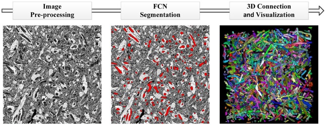
Figure 1
The pipeline of our proposed method. (Left to Right) Image pre-processing with registration and histogram equalization; mitochondria segmentation with the proposed 3D residual FCN; 3D connection and v...

Figure 2
Illustration of the datasets. (A) Isotropic image from mouse hippocampus obtained by FIB-SEM; (B) Ground truth of the FIB-SEM image; (C) Anisotropic image from rat cortex acquired by ATUM-SEM; (D) Gro...
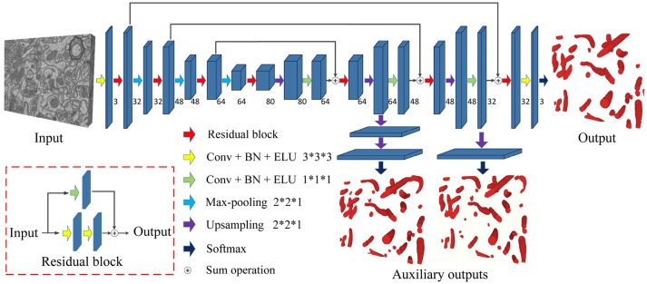
Figure 3
The architecture of the proposed network. Blue blocks denote feature maps, and numbers imply the channel of feature maps in each layer. The red arrow represents the residual block, which consists of t...
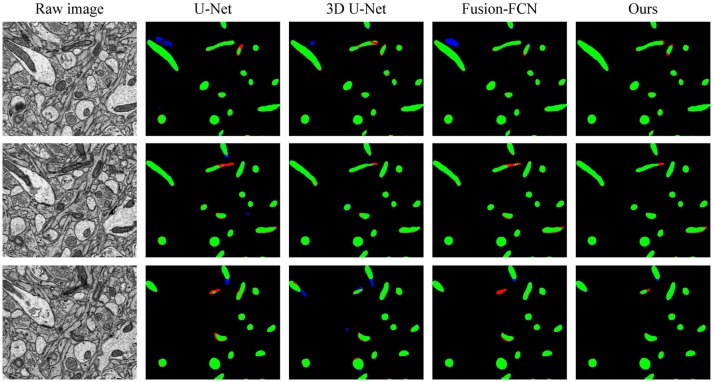
Figure 4
The qualitative comparisons between different methods in three continuous sections from the ATUM-SEM dataset. Green pixels denote TP, red pixels denote FN, blue pixels indicate FP and black pixels den...

Figure 5
The qualitative comparisons between different methods on the FIB-SEM dataset. Note that our method significantly reduces the number of FNs (red) and FPs (blue).
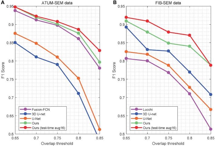
Figure 6
Detection performance of the different overlap thresholds on both EM datasets. Our approach achieves better performance than that of the baseline approaches. (A) ATUM-SEM dataset. (B) FIB-SEM dataset.

Figure 7
3D reconstruction of mitochondria. (A) Reconstruction of mitochondria from the ATUM-SEM dataset with a volume of 15.2 u00d7 17.2 u00d7 8.9 u03bcm 3 ; (B) Reconstruction of mitochondria from the FIB-SE...
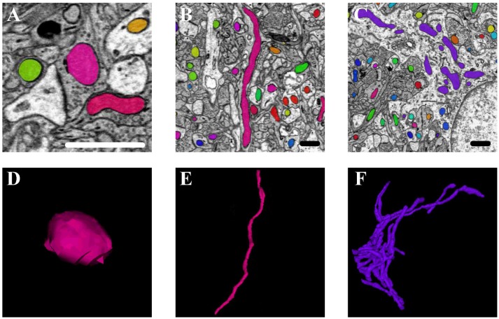
Figure 8
The 3D morphology of mitochondria in different positions in the neurons. (A,D) The mitochondria (in pink) positioned at sites of synapse; (B,E) the mitochondria (in pink) located in the axons and dend...
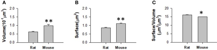
Figure 9
Measurement of the mitochondrial statistics in mouse cortex and rat hippocampus. (A) Measurement of the mitochondrial volume in mouse cortex and rat hippocampus. (B ) Measurement of the mitochondrial ...
Figure images are served from the NIH/NLM PubMed Central Open Access Subset or Europe PMC; copyright remains with the publishers and authors.
💬 Discussion
0 commentsNo comments yet. Be the first to start a discussion!
Leave a Comment