Abstract
AbstractDigital holographic microscopy enables the 3D reconstruction of volumetric samples from a single-snapshot hologram. However, unlike a conventional bright-field microscopy image, the quality of holographic reconstructions is compromised by interference fringes as a result of twin images and out-of-plane objects. Here, we demonstrate that cross-modality deep learning using a generative adversarial network (GAN) can endow holographic images of a sample volume with bright-field microscopy contrast, combining the volumetric imaging capability of holography with the speckle- and artifact-free image contrast of incoherent bright-field microscopy. We illustrate the performance of this “bright-field holography” method through the snapshot imaging of bioaerosols distributed in 3D, matching the artifact-free image contrast and axial sectioning performance of a high-NA bright-field microscope. This data-driven deep-learning-based imaging method bridges the contrast gap between coherent and incoherent imaging, and enables the snapshot 3D imaging of objects with bright-field contrast from a single hologram, benefiting from the wave-propagation framework of holography.
🔬 Techniques
🔭 Microscopes
💻 Software
🏭 Microscope Brands
🔎 Objectives
💻 Software Details
🏛️ Research Organizations (ROR)
Affiliated research institutions:
📋 Methods
Digital holographic image acquisition
The holographic images were acquired using a customized lens-free imaging system (see Supplementary Fig. S5 for details). The system consisted of a vertical-cavity surface-emitting laser diode ( λ = 850 nm) for illumination, a complementary metal–oxide–semiconductor image sensor (Sony IMX219PQ, 1.12-µm pixel size), and a Raspberry Pi 2 for system control. This near-infrared illumination was chosen to enable the use of all four Bayer channels of the color image sensor chip to improve the pixel-size-limited resolution of the hologram that could be achieved in a single snapshot. The sample was mounted on a 3D-printed sample holder placed ~500 µm above the image sensor surface. The illumination source was placed ~8 cm above the sample plane without any additional spatial or spectral filter.
Scanning bright-field microscopy image acquisition and alignment
The bright-field microscopy images were captured by an inverted scanning microscope (IX83, Olympus Life Science) using a 20 × 0.75 NA objective lens (UPLSAPO20X, Olympus Life Science). The microscope scanned each sample at different lateral locations, and at each location, an image stack of −30 to 30 µm with a 0.5-µm step size was captured. After the capture of these bright-field images, the microscopy image stack was aligned using the ImageJ plugin StackReg 25 , which corrected the rigid shift and rotation caused by the inaccuracy of the microscope scanning stage. Hologram backpropagation and autofocusing The raw digital in-line hologram was balanced and shade corrected by estimating the low-frequency shade of each Bayer channel using a wavelet transform 26 . This corrected hologram was digitally backpropagated to different planes (which matched the corresponding planes in the bright-field microscopy image stack) using angular-spectrum-based free-space backpropagation 4 , 27 . For this purpose, 3× padding was used in the angular-spectrum (Fourier) domain, which effectively interpolated the hologram pixel size by 3×. To match the heights of the backpropagated holograms and the corresponding bright-field microscopy image stacks, the focal planes were estimated and cross-registered as “zero” height, and the relative axial propagation distance was determined to match the axial scanning step size of the bright-field microscope (0.5 µm). The digital hologram’s focal plane was estimated using an edge sparsity-based holographic autofocusing criterion 28 . Network and training The GAN implemented here consisted of a generator network and a discriminator network, as shown in Supplementary Fig. S1 . The generator network employed a variation of the original U-Net 29 design with minor modifications and additional residual connections 30 . The discriminator network was a convolutional neural network with six convolutional blocks and two fully connected (linear) layers. The original training data consisted of ~6000 image pairs (see Supplementary Table S2 for details), which were augmented to 30,000 image pairs by random rotation and flipping of the images. The validation data were not augmented. In each training iteration, the generator network was updated six times using the adaptive moment estimation (Adam) optimizer with a learning rate of 10 − 4 , whereas the discriminator network was updated three times with a learning rate of 3 × 10 −5 . The validation set was tested every 50 iterations, and the best network was chosen to be the one with the lowest mean absolute error loss on the validation set. The network was built using an open-source deep-learning package, TensorFlow 31 . The training and inference were performed on a PC with a six-core 3.6-GHz CPU and 16 GB of RAM using an Nvidia GeForce GTX 1080 Ti GPU. On average, the training process took ~90 h for ~50,000 iterations (equivalent to ~40 epochs). After training, the network inference time was ~0.1 s for an image patch of 256 × 256 pixels (see the Supplementary Information for details ).
Show full methods section
Digital holographic image acquisition
The holographic images were acquired using a customized lens-free imaging system (see Supplementary Fig. S5 for details). The system consisted of a vertical-cavity surface-emitting laser diode ( λ = 850 nm) for illumination, a complementary metal–oxide–semiconductor image sensor (Sony IMX219PQ, 1.12-µm pixel size), and a Raspberry Pi 2 for system control. This near-infrared illumination was chosen to enable the use of all four Bayer channels of the color image sensor chip to improve the pixel-size-limited resolution of the hologram that could be achieved in a single snapshot. The sample was mounted on a 3D-printed sample holder placed ~500 µm above the image sensor surface. The illumination source was placed ~8 cm above the sample plane without any additional spatial or spectral filter.
Scanning bright-field microscopy image acquisition and alignment
The bright-field microscopy images were captured by an inverted scanning microscope (IX83, Olympus Life Science) using a 20 × 0.75 NA objective lens (UPLSAPO20X, Olympus Life Science). The microscope scanned each sample at different lateral locations, and at each location, an image stack of −30 to 30 µm with a 0.5-µm step size was captured. After the capture of these bright-field images, the microscopy image stack was aligned using the ImageJ plugin StackReg 25 , which corrected the rigid shift and rotation caused by the inaccuracy of the microscope scanning stage. Hologram backpropagation and autofocusing The raw digital in-line hologram was balanced and shade corrected by estimating the low-frequency shade of each Bayer channel using a wavelet transform 26 . This corrected hologram was digitally backpropagated to different planes (which matched the corresponding planes in the bright-field microscopy image stack) using angular-spectrum-based free-space backpropagation 4 , 27 . For this purpose, 3× padding was used in the angular-spectrum (Fourier) domain, which effectively interpolated the hologram pixel size by 3×. To match the heights of the backpropagated holograms and the corresponding bright-field microscopy image stacks, the focal planes were estimated and cross-registered as “zero” height, and the relative axial propagation distance was determined to match the axial scanning step size of the bright-field microscope (0.5 µm). The digital hologram’s focal plane was estimated using an edge sparsity-based holographic autofocusing criterion 28 . Network and training The GAN implemented here consisted of a generator network and a discriminator network, as shown in Supplementary Fig. S1 . The generator network employed a variation of the original U-Net 29 design with minor modifications and additional residual connections 30 . The discriminator network was a convolutional neural network with six convolutional blocks and two fully connected (linear) layers. The original training data consisted of ~6000 image pairs (see Supplementary Table S2 for details), which were augmented to 30,000 image pairs by random rotation and flipping of the images. The validation data were not augmented. In each training iteration, the generator network was updated six times using the adaptive moment estimation (Adam) optimizer with a learning rate of 10 − 4 , whereas the discriminator network was updated three times with a learning rate of 3 × 10 −5 . The validation set was tested every 50 iterations, and the best network was chosen to be the one with the lowest mean absolute error loss on the validation set. The network was built using an open-source deep-learning package, TensorFlow 31 . The training and inference were performed on a PC with a six-core 3.6-GHz CPU and 16 GB of RAM using an Nvidia GeForce GTX 1080 Ti GPU. On average, the training process took ~90 h for ~50,000 iterations (equivalent to ~40 epochs). After training, the network inference time was ~0.1 s for an image patch of 256 × 256 pixels (see the Supplementary Information for details ).
Supplementary information Supplementary Information Movie 1. Bright-field holographic imaging of a 3D pollen stack using our deep learning-based inference and its comparison to a scanning bright-field microscope
📊 Figures
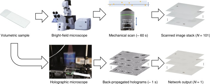
Fig. 1
Bright-field holography.
High-contrast bright-field imaging of a volumetric sample requires mechanical axial scanning and the acquisition of many successive images (e.g., N =u2009101 here spansu2009u00b1u2009500u2009u00b5m in...
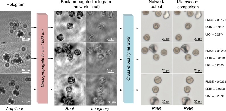
Fig. 2
Imaging of a pollen mixture captured on a substrate.
Each input hologram is shown with a larger FOV to better illustrate the fringes. Each network output image is quantitatively compared against the corresponding bright-field microscopy ground-truth ima...
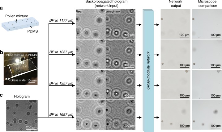
Fig. 3
Use of cross-modality deep learning in bright-field holography to fuse the volumetric imaging capability of holography with the speckle- and artifact-free image contrast performance of incoherent bright-field microscopy.
The pollen sample is dispersed in 3D throughout a bulk volume of PDMS (thickness ~800u2009u00b5m). BP: digital backpropagation. Also see Movie 1
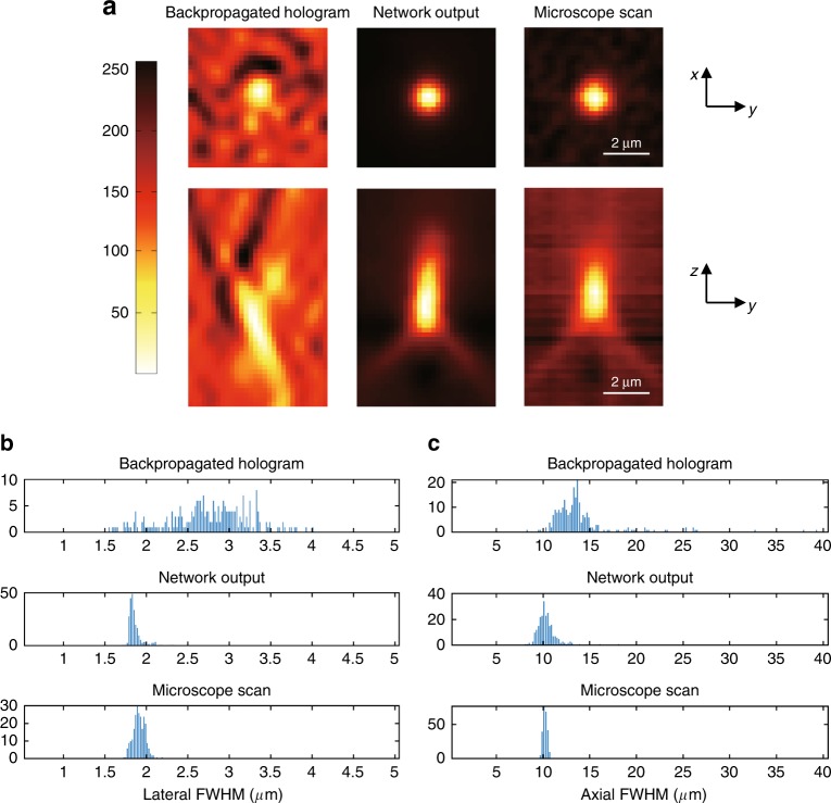
Fig. 4
3D PSF comparison using 1-u03bcm beads.
a 3D imaging of a single microbead and a comparison of the standard holographic backpropagation results against the network output and the images captured by a scanning bright-field microscope via N =...
Figure images are served from the NIH/NLM PubMed Central Open Access Subset or Europe PMC; copyright remains with the publishers and authors.
💬 Discussion
0 commentsNo comments yet. Be the first to start a discussion!
Leave a Comment