Abstract
Neuroblastoma (NB) is one of the most frequently occurring cancerous tumors in children. The current grading evaluations for patients with this disease require pathologists to identify certain morphological characteristics with microscopic examinations of tumor tissues. Thanks to the advent of modern digital scanners, it is now feasible to scan cross-section tissue specimens and acquire whole-slide digital images. As a result, computerized analysis of these images can generate key quantifiable parameters and assist pathologists with grading evaluations. In this study, image analysis techniques are applied to histological images of haematoxylin and eosin (H&E) stained slides for identifying image regions associated with different pathological components. Texture features derived from segmented components of tissues are extracted and processed by an automated classifier group trained with sample images with different grades of neuroblastic differentiation in a multi-resolution framework. The trained classification system is tested on 33 whole-slide tumor images. The resulting whole-slide classification accuracy produced by the computerized system is 87.88%. Therefore, the developed system is a promising tool to facilitate grading whole-slide images of NB biopsies with high throughput.
💻 Software
🧪 Sample Preparation
🏭 Microscope Brands
💻 Software Details
🏛️ Research Organizations (ROR)
Affiliated research institutions:
📋 Methods
2.1.
Image acquisition
In this study, all NB tumor slides are collected from Nationwide Children’s Hospital in accordance with an Institutional Review Board (IRB) protocol. According to the protocols commonly used in the Children’s Oncology Group, these tissue slides are cut at a thickness of 5 μm and soaked in paraffin at the preparation stage. Each NB slide in the dataset is prepared using a dual staining procedure in which haematoxylin and eosin (H&E) are used to increase the visual contrasts among different cytological components. After being stained with H&E, each thin tissue slide is then fixed on a scanning bed and digitized using ScanScope T2 digitizer (Aperio, San Diego, CA) at 40× magnification, allowing for clear visualization of tumor architectures. The resulting whole-slide images are quite large with their sizes up to 40 GB. Due to the limited hardware storage capability, the resulting digital images are compressed following the JPEG compression standards at approximately a 1:40 compression ratio. After the compression, the typical image sizes can vary from 1 to 4 GB. To make the image analysis more tractable, we partition each histology slide image into multiple non-overlapping image tiles of the size 512 × 512 in pixels, rather than requiring our classification system to work on the whole-slide image. Another benefit of breaking down whole-slide images into tiles is that we can make full use of the distributed computational infrastructure. The parallel implementation details will be discussed in Section 2.3. 2.2.
Show full methods section
2.1.
Image acquisition
In this study, all NB tumor slides are collected from Nationwide Children’s Hospital in accordance with an Institutional Review Board (IRB) protocol. According to the protocols commonly used in the Children’s Oncology Group, these tissue slides are cut at a thickness of 5 μm and soaked in paraffin at the preparation stage. Each NB slide in the dataset is prepared using a dual staining procedure in which haematoxylin and eosin (H&E) are used to increase the visual contrasts among different cytological components. After being stained with H&E, each thin tissue slide is then fixed on a scanning bed and digitized using ScanScope T2 digitizer (Aperio, San Diego, CA) at 40× magnification, allowing for clear visualization of tumor architectures. The resulting whole-slide images are quite large with their sizes up to 40 GB. Due to the limited hardware storage capability, the resulting digital images are compressed following the JPEG compression standards at approximately a 1:40 compression ratio. After the compression, the typical image sizes can vary from 1 to 4 GB. To make the image analysis more tractable, we partition each histology slide image into multiple non-overlapping image tiles of the size 512 × 512 in pixels, rather than requiring our classification system to work on the whole-slide image. Another benefit of breaking down whole-slide images into tiles is that we can make full use of the distributed computational infrastructure. The parallel implementation details will be discussed in Section 2.3. 2.2.
Image dataset
The image dataset used in this study consists of 36 NB cases, covering all three subtypes of neuroblastic grading. All tumor slides are selected in such a way that they are good representatives of different grade subtypes and contain a sufficiently large number of cytological components of interest in the tissue regions. In our study, the training dataset consists of 389 image tiles of the size 512×512 in pixels, equally selected at random from three representative cases (one from each subtype). The remaining 33 case images from the dataset are used for the testing purpose. The images in our database are evaluated by an experienced pathologist who visually categorized them into three distinctive differentiation grades. The average storage size of testing slides is about 20 GB before compression, which approximately corresponds to 27,400 image tiles of 512 × 512 pixels in size. 2.3.
Software and hardware
The developed classification algorithm and the graphical user interface are designed using MATLAB (The MathWorks, Inc., Natick, MA). All experimental evaluations of our work are carried out on a 64-node cluster with Linux OS owned by the Department of Biomedical Informatics at The Ohio State University. Each node of the cluster is equipped with dual 2.4 GHz Opteron 250 processors, 8 GB of DDR400 RAM with 1 GB dimms and a 250 GB SATA hard disk. The computation infrastructure is designed with a master–client architecture in which a master application and multiple client applications work in a collaborative pattern [ 9 ]. For each computation task, one master node is responsible for partitioning the tumor slide images into image tiles with a fixed size and distributing data to clients for further processing in a round-robin fashion. Each client keeps local copies of the assigned image tiles and initiates a local MATLAB application to analyze the cached image tiles with the developed classification algorithm. Once the automated image analysis process ends, the master node is, again, in charge of collecting classification results from client nodes and re-assembles them in order before it produces the grading classification results over the whole-slide images. 2.4. Multi-resolution paradigm Multi-resolution analysis has shown its power in many computer-aided diagnosis (CAD) systems, as CAD systems usually involve processing a large volume of medical image data with prohibitive computational costs. In the work presented by Liang and Page [ 10 ], they addressed the problem of demanding computations by adjusting the weights in the neural network with a multi-resolution strategy. Yu et al. took the similar idea and used a hierarchical clustering method to obtain the coarse-to-fine classifiers from a clustering tree [ 11 ]. Furthermore, a multi-resolution classification model was proposed by He et al. who classified data using the support vector machines (SVM) in a multi-resolution classification model [ 12 ]. In another histopathological image analysis application, Doyle et al. performed pixel-wise Bayesian binary classification at each image resolution level to produce the likelihood scenes from selected regions of interest [ 8 ]. Our CAD system for discriminating the grade of neuroblastic differentiation makes full use of the multi-resolution principle in that the system emulates the way pathologists examine histology slides with different magnifications. In accordance with the coarse-to-fine strategy, the developed classification system begins analyzing images at the lowest image resolution level. Processing at higher resolution levels is only invoked when the classification performance associated with the lower resolution level is not sufficient. At each image resolution level, a complete and automated analysis pipeline is followed. As shown in Fig. 3 , the sequence of processes include image–tile generation, establishment of the multi-resolution hierarchy, color conversion, clustering-based segmentation, feature construction, feature selection, dimensionality reduction, multi-classification, classifier combination, and performance evaluation [ 13 ]. As the initial step of the whole process, each image tile analyzed by the computerized system is decomposed into a set of image representations in such a way that the lower resolution image contains most of the relevant image details from higher resolution levels. Let us denote I L [ n , m ] as the input image tile at the full resolution, where L is the number of resolution hierarchies. The image versions with a sequence of resolutions can be represented by (1) S ( I ) = { I l [ n , m ] | l = 1 , 2 , … , L − 1 ; and [ n , m ] ∈ Z N l × Z M l } where I l [ n , m ] is the image that is down-sampled for L−l times from the full resolution copy I L [ n , m ]; Z N l and Z M l are the integer fields associated with row and column directions at the revolution level l ; N l and M l , respectively, designate the row number and the column number of I l [ n , m ]. For each down-sampling process, we follow such a method that the output image is a non-aliasing version in the spatial frequency domain of the next higher resolution tile. This process can be mathematically expressed as (2) F l [ k , s ] = ∑ n = 0 N l − 1 ∑ m = 0 M l − 1 I l [ n , m ] W N l n k W M l m s where W N l = e − j ( 2 π / N l ) and W M l = e − j ( 2 π / M l ) . In Eq. (2) , F l [ k , s ] is the two-dimensional discrete Fourier transform of I l [ n , m ]. Although there is no particular reason to claim that I l [ n , m ] has a limited bandwidth, we can in general run an ideal window filter and truncate its bandwidth in the spatial frequency domain: (3) G l [ k , s ] = F l [ k , s ] H l [ k , s ] The ideal low pass filter H l [ k , s ] is defined as (4) H l [ k , s ] = { 1 ( k − N l 2 ) 2 + ( s − M l 2 ) 2 < α 2 min ( N l , M l ) 0 otherwise where α(≤ 1) is the size reduction factor. In our application, α = 0.5. Therefore, the resulting down-sampled image can be obtained by taking the inverse Fourier transform of the non-zero response area in H l [ k , s ]. The designed algorithm initially examines the image tiles at the lowest resolution that corresponds to the lowest optical magnification under the microscope. The lower-resolution image is scaled by a factor of two on each image dimension, thus a quarter as large as the image tile of the next higher resolution level. In our tests, a four layered multi-resolution hierarchy is built up, with {(512×512), (256×256), (128 × 128), (64 × 64) as the set of tile sizes from the highest to the lowest resolution, respectively. An example of image resolution hierarchy with its resolution decreased from the bottom to the top level is shown in Fig. 4 , where L = 4. Since the lowest resolution images are the smallest ones in size within the image representation hierarchy, it requires the least amount of time to process these images. However, if the images at lower resolution levels do not contain sufficient image details, the computerized system automatically switches to work on images at the next higher resolution. As a result, the dynamic change across images of different resolution levels is an analogy to the way a pathologist adjusts the microscope magnification based on the amount of details needed to analyze a particular portion of a tumor slide. 2.5.
Image segmentation
At each resolution level, each image is segmented into multiple cytological components necessary for further analysis. Although there are large variations of tissue architectures in images of NB samples having different differentiation grades, five salient components (nuclei, cytoplasm, neuropil, red blood cells (RBCs), and background) can usually be discerned. Additionally, relatively discriminating color contrasts enhanced by the H&E staining process provide us many useful image clues. For example, nuclei and cytoplasm regions are stained with blue-purple in color while regions with pink and red hues suggest neuropils. As a result, it is promising to develop a clustering-based segmentation analysis that identifies different cytological components in a well-formulated feature space. Guided by these ideas, we develop a novel segmentation method, namely EMLDA [ 14 ], that works in a feature space constructed with combined color and entropy information extracted from the RGB and the La * b * image channels. The La * b * color space is developed by the Commission Internationale d’Eclairage (CIE) [ 15 ]. When it is compared to other color spaces such as HSI, YIQ, and YUV, it presents the desired color perceptual uniformity that allows the use of Euclidean distance metric rational. The La * b * color space is also a good choice in terms of its ability to represent luminance and chrominance information separately. By its definition, channel L carries the information for the light intensity while color information is contained in a * and b * components. As a supplement, three entropy statistics computed with a 9 × 9 window shifting across the R, G, and B image components are used to enrich the feature vector. Our novel segmentation approach integrates the Fisher–Rao criterion into the generic expectation–maximization algorithm and iteratively partitions data in the resulting feature space in such a way that the data associated with different classes can be separated as much as possible. This process is repeated until the Fisher–Rao criterion, the ratio of the sum of squared between-class distances to the sum of squared within-class distances, converges to its maxima. Suppose C components are to be segmented from a given image. Let us denote X = { x | x ∈ ℛ p } as the dataset in a p -dimensional feature space. The expectation and maximization step of the EMLDA method can then be summarized as follows. E step (expectation): Find the optimal projection matrix: (5) V ∗ = arg max V ∈ R p × s J ( V | θ ) = arg max V ∈ R p × s | V T S B ( θ ) V | | V T S W ( θ ) V | where J ( V | θ ) is the Fisher–Rao criterion to be maximized. V * is a p×s matrix consisting of s discriminant vectors as its columns, where s ≤ C −1. In addition, θ , is the labelling configuration determined from the previous step, while S B and S W are the between- and within-class scatter matrices that are symmetric and positive-definite [ 16 ]. M step (maximization): The matrix V * maximizing the Fisher–Rao criterion J ( V | θ ) is composed of s column-wise discriminant feature vectors onto which the set of data X are projected. By x ∼ T = x T V ∗ , the projected data X ∼ = { x ∼ | x ∼ ∈ ℛ s } are mapped to a lower dimensional space where the data associated with the C classes can be best discriminated. Next, find: (6) θ ∼ = arg max i ∈ Θ ( − ‖ x ∼ − m ∼ i ‖ 2 ) Where Θ = {1, 2,…, C } is the label set; m i and m ∼ i are the means of class i in the original and reduced dimensional feature space that are related by m ∼ i = m i T V ∗ . After finding the labels θ ∼ for all data points, we substitute θ with θ ∼ and repeat steps (1) and (2) again, until J ( V * | θ ) converges to a local maximum. One beauty associated with this method is that one can simply skip the feature normalization step due to the following theorem. Theorem 1 Feature normalization by linear scaling to unit range does not change the end classification result with EMLDA. Proof of Theorem 1 Suppose the mapping functions are linear scaling transformations that map each feature x to a specific unit range, i.e., x ^ = M x + D , where M = diag( m 11 ,…, m pp ) and D = ( d 1 ⋯ dp ) T , then the between-class scatter matrix in the transformed data space is (7) S ^ B = ∑ i = 1 C n i ( m ^ i − m ^ ) ( m ^ i − m ^ ) T = ∑ i = 1 C n i ( ( M m i + D ) − ( M m + D ) ) ( ( M m i + D ) − ( M m + D ) ) T = ∑ i = 1 C n i M ( m i − m ) ( m i − m ) T M T = M S B M T = M T S B M where m is the overall mean and n i is the number of samples of class i . Similarly, we have the within-class scatter matrix in the transformed data space as S ^ W = M T S W M Furthermore, we have (8) J ^ ( V ^ ) = V ^ T S ^ B V ^ V ^ T S ^ W V ^ = V ^ T M T S B M V ^ V ^ T M T S W M V ^ = J ( V ) where V = M V ^ . Eq. (8) reveals the fact that J and J ^ can be simultaneously maximized when V ∗ = M V ^ ∗ . The projected and the mean in the lower dimension space spanned by the discriminant vectors for X = { x|x ε R p } are x T V * and m i T V ∗ , while those associated with X ^ = { x ^ | x ^ ∈ R p } are (9) x ^ T V ^ ∗ = ( M x + D ) T V ^ ∗ = x T M V ^ ∗ + D T V ^ ∗ = x T V ∗ + D T V ^ ∗ m ^ i T V ^ ∗ = ( M m i + D ) T V ^ ∗ = m i T M V ^ ∗ + D T V ^ ∗ = m i T V ∗ + D T V ^ ∗ i.e., the projected data derived from X and X ^ are related by a simple translation. Therefore, the end classification results in X and X ^ feature space are conserved to be the same. ■ In our study, we define four classes: nuclei, cytoplasm, neuropils, and background (i.e., C = 4). Given the fact that RBCs may occupy a large area within image tiles, a simple yet efficient threshold-based method is used to identify the RBC regions before the iterations are initiated. As a result, the number of defined classes is kept as low as possible, which contributes to the reduction of time costs. A set of segmentation results on a typical image tile associated with the UD grade are shown in Fig. 5 , which verifies the effectiveness of this segmentation approach. 2.6. Feature construction Although pathologists tend to rely heavily on morphologic features such as nuclear size and cellularity, a large amount of information derived from textures of different histological structures is integrated into their decision procedures in an implicit way [ 17 ]. By creating the feature vector, it is our intention to input into the computerized system information that helps discriminate different pathological components effectively. Therefore, in our implementation, all features are derived from color information and textural patterns as they depend less on the segmentation accuracy. In our study, local statistical measures are computed only from the segmented regions associated with cytoplasm and neuropils identified by the proposed segmentation algorithm in that they usually bear texture patterns considerably distinct across tumor tissues of different grades. Associated with cytoplasm and neuropil regions, four textural Haralick features [ 18 ] are computed: the entropy, mean, and variance of the range of values within a local neighborhood, and the homogeneity degree of the co-occurrence matrix in L , a * and b * channels. As a result, a feature vector composed of 24 elements is constructed as a symbolic representation of each image tile. For comparison, summaries of the set of features used by pathologists and those employed in the computerized system are reported in Tables 1 and 2 , where two apparent distinctions can be observed. Pathologists tend to use morphological and pathological characteristics in their prognosis, while the computer system prefers using statistical features. The characteristics used by pathologists are qualitative, as opposed to the quantitative features utilized by the computer system. 2.7.
Feature selection and classification
Although we use a vector of features to characterize the texture patterns of cytological structures, it is not the case, in general, that each extracted feature component contributes to the characterization of the texture patterns. More importantly, they may not increase the classification accuracy in equal proportions. Some features may contain far more discriminating information than others. By contrast, some other features may contribute less in improving the classification accuracy. The choice of the most discriminating subset of features is not only conducive to substantial reduction in computational complexity, but it also leads to improved classification accuracies. In fact, if more than the necessary number of features are used, the classification performance can deteriorate due to the “peaking phenomenon” [ 16 ]. As a result, we are interested in seeking out the best subset of features that yield the best classification accuracy and have the least number of members. In our application, the subset of features sufficient for classifying well-organized data are determined by a popular feature selection technique, namely the sequential floating forward selection (SFFS) procedure [ 19 ]. The SFFS procedure is an upgraded version of the sequential selection procedures with back-tracking mechanisms, such as plus l − take away r algorithm. In addition to these methods, the number of forward and backtracking steps (i.e., l and r ) in SFFS are dynamically adjusted rather than fixed values set in advance. In other words, SFFS allows a dynamic number of features that have been selected to be removed in a dynamic number of posterior steps. As a result, SFFS is very efficient and effective even on problems of high dimensionality with non-monotonic feature selection criterion functions. Since our proposed multi-resolution hierarchy has four resolution levels, the optimal subset of features needs to be determined with training image tiles from each resolution layer. This is due to the fact that neither histopathological nor statistical characteristics of image tiles across different resolution levels are necessarily the same. In practice, they could be considerably distinct from each other. As a result, the ensuing subset of selected features may not be the same when computed at different resolutions. After the optimal subsets of features extracted from the training data associated with different resolutions are obtained in the training phase, we can establish the new feature vectors with only those feature components selected in the training process and classify the feature data in a lower dimensional feature space in the testing stage. Furthermore, the feature selection process is carried out in combination with different classifiers over all the training data in an offline pattern. To achieve a good classification performance, multiple classifiers were employed: K-nearest neighbor (KNN), linear discriminant analysis (LDA) & KNN, LDA & nearest mean (NM), correlation LDA (CORRLDA) [ 20 ] & KNN, CORRLDA & NM, LDA & Bayesian and SVM [ 21 ] with a linear kernel. KNN is a very intuitive classifier that assumes observations associated with the same class label are close to each other measured by some metric in a feature space. Assuming { x 1 , x 2 ,…, x k } is a set consisting of the nearest K observations, under the distance}metric d (. , .), to the given data x whose class label is to be determined, the class·label of x is the majority vote of the nearest K neighbors. Likewise, NM classifier assigns data to the class associated with the closest class mean. Unlike the non-parametric classifiers, Bayesian classifier can reach the optimal recognition result given that all underlying true class-conditional probability density functions are known. Another useful classifier widely used n machine learning process is known as SVM that can deal with non-linearly separable cases by mapping data from a lower dimensional space to a higher dimensional one where data becomes linearly separable. In addition to the four classifiers, two feature extraction methods, i.e., LDA and CORRLDA, are used in combination with the classifiers in reducing the dimensionality of the feature space. LDA aims at finding the best subspace where the between-class variance is maximized while the within-class variance is minimized. However, it does not necessarily guarantee the minimum Bayes error of the given data distributions when the eigenvectors associated with the largest eigenvalues of the between-class scatter matrix have a high correlation with the most principal eigenvectors of the within-class scatter matrix. By contrast, CORRLDA is a method to select the most discriminative eigenvectors of the within-class scatter matrix that is often singular. Rather than picking up the most principle eigenvectors, it keeps the eigenvectors that are most correlated to the bases spanning the range space of the between-class scatter matrix. For more detailed discussions on these methods, readers are referred to [ 16 , 20 , 21 ]. As different feature extraction approaches and classifiers are optimal under different assumptions, no single combination of one specific dimensionality reduction technique and one fixed classifier can guarantee the best feature representation and the resulting minimum Bayes error in the absence of assumptions on feature distributions. As a result, no general algorithm exists that can always achieve superior recognition rates to those of others under all possible circumstances. However, one feasible way to boost the system classification performance is to use a collection of classifiers, rather than a single one. It has been shown that the overall error rate decreases monotonically as more classifiers are used in a system, as long as each individual classifier has an error rate less than random guessing [ 22 ]. As each classifier has its own feature regions where it yields the best performance, a combination of classifiers can achieve higher classification accuracies in theory. As a result, the ensemble classification system comprising seven classifiers is developed for the decision-making component. Since the seven classifiers included in this classification group present different characteristics and various classification mechanisms, aggregation of these classifiers can help improve the end recognition performances. 2.8. Classifier combiner To make full use of the group of classifiers, a combination strategy is proposed to combine those decisions made by the collection of classifiers in a parallel pattern. Although a number of architectures for classifier combination have been proposed, such as the dynamic classifier selection (DCS), classifier hierarchical concatenation (CHC), and serial combination (SC), we choose to aggregate the outputs of the multiple classifiers with a straightforward two-step classifier combining mechanism that consists of a voting and weighting procedure. This is due to the fact that a sum rule-based combination paradigm outperforms the others in general [ 23 ]. The combining mechanism can be described in the following two steps. Step 1: The combiner evaluates the outputs of all K classifiers ( K = 7 in this work) and produces a final decision θ * that refers to the decisions supported by the majority of the K classifiers: (10) θ ∗ = arg max i ∈ { 1 , 2 , … , C } Ψ ( i ) where Ψ ( i ) is the number of votes for the i th class collected from the K classifiers and C is the number of classes ( C = 3 in this work). Step 2: We next evaluate the confidence degree of the voted classification result at the current resolution level. Since the combination scheme of the sum rule is usually superior to the others, the confidence degree in this study is defined as the sum of weights assigned to classifiers that concur with the combiner. The corresponding weight assigned to each classifier, in each resolution level, is computed by normalizing the priori classification accuracies of all the classifiers over the training data with the leave-one-out validation process. The higher the priori classification accuracy one classifier has, the more biased it is weighted. If the sum of weights of the classifiers whose decisions concur with each other is greater than a given threshold, the ensemble decision supported by the majority of classifiers is accepted as an end result. Otherwise, the system switches to work on the image version at the next higher resolution level where the same sequence of image processing steps are followed again. In summary, the hypothesis test and the resulting decision rule can be written as H 0 : classification result is good enough ; quit the process ; H 1 : go to the next higher resolution level for classification ; Decision = { H 0 if S l ⩾ γ l , l + 1 l = 1 , 2 , 3 H 1 otherwise where (11) S l = ∑ i = 1 k w l ( i ) ∑ j = 1 k w l ( j ) δ θ ( i ) , θ ∗ In Eq. (11) , w l ( i ) is the priori recognition rate of the classifier i at resolution level l ; δ i , j is the Kronecker delta function; θ ( i ) is the class label decided by the classifier i ; γ l , l+ 1 is the threshold of the confidence measure with which the system decides whether or not it needs to proceed with further analysis from image resolution l to l + 1.
📊 Figures
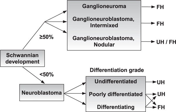
Fig. 1
A simplified tree diagram of the International Neuroblastoma Pathology Classification (the Shimada system), where UH represents u201cunfavorable histologyu201d and FH stands for u201cfavorable histolo...
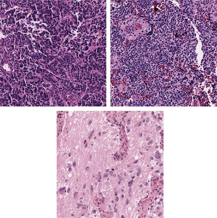
Fig. 2
Typical tissue images associated with the three differentiation grades: (a) undifferentiated grade, (b) poorly-differentiated grade, and (c) differentiating grade.
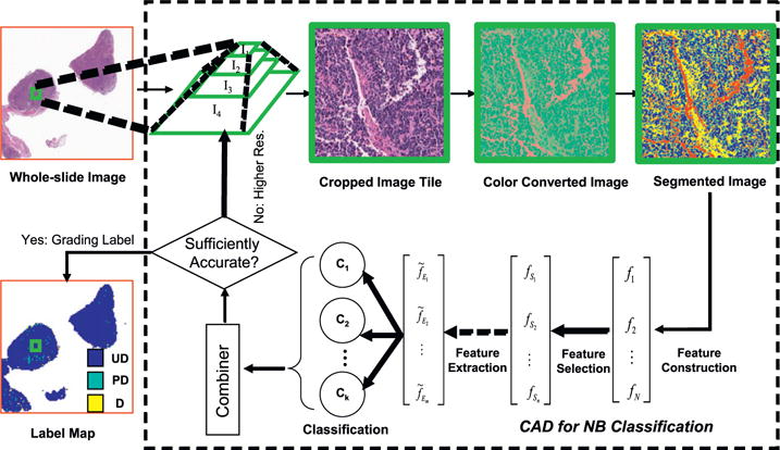
Fig. 3
Flowchart of the developed image processing system. A whole-slide image of a neuroblastoma tumor with its size of 59, 412u00d764, 990 in pixels (13, 932 u03bcmu00d715, 183u03bcm) is processed with ste...
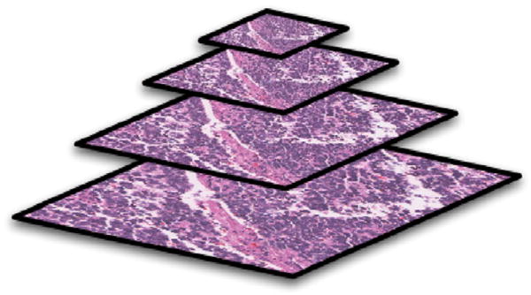
Fig. 4
A typical example of the multi-resolution representation hierarchy with image sizes scaled by half at each dimension from bottom to top resolution level.
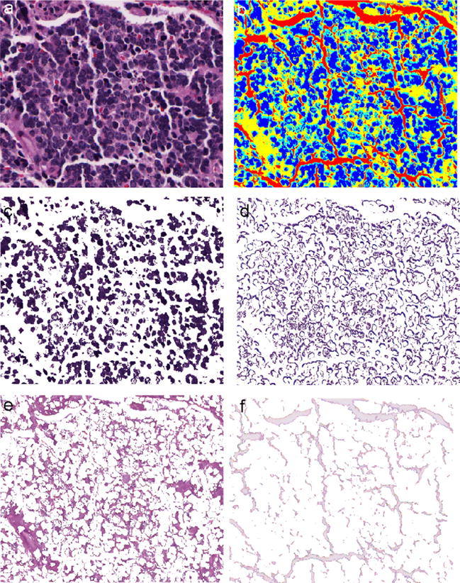
Fig. 5
The segmented components in a typical image from undifferentiated subtype are shown. (a) Original image. (b) Partitioned image shown in colors with nuclei in blue, cytoplasm in cyan, neuropil in yello...
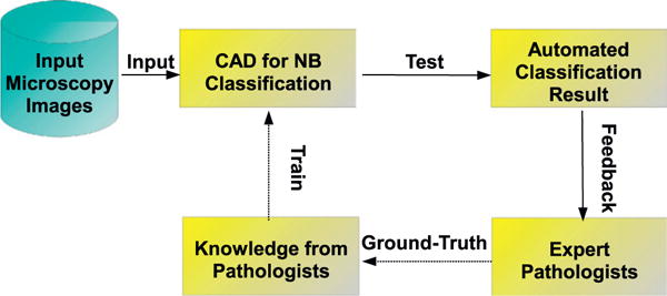
Fig. 6
Flowchart of the developed classification system. The solid arrows indicate online steps and the dashed arrows indicate offline steps.
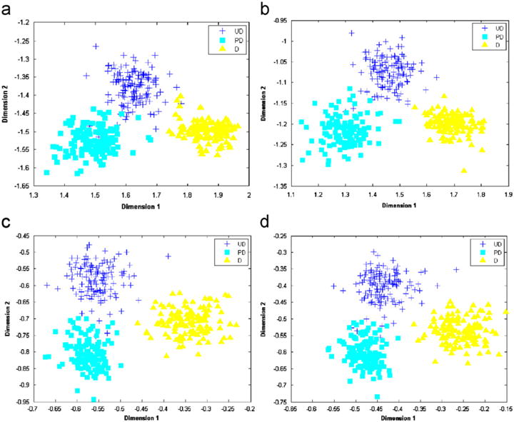
Fig. 7
Scatter plots of the training features in a two-dimensional feature space associated with four resolution levels (from the lowest to highest) are shown in (a)u2013(d). These features are selected and ...
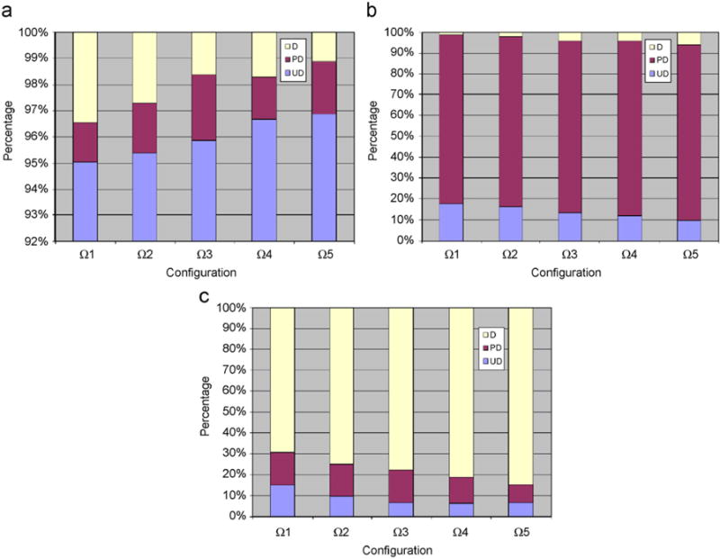
Fig. 8
Percentages of image tiles graded as undifferentiated, poorly differentiated, and differentiating for the three testing slides (i.e., Nos. 1u20133 in Table 6 ) are shown in (a)u2013(c), respectively. ...
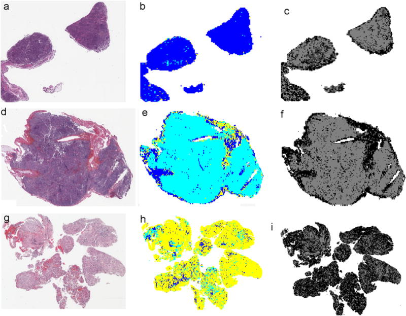
Fig. 9
Image tile-level classification results of three typical tumor slides using configuration u03a9 5 are shown. (a), (d), and (g) are the H&E stained whole-slide images classified as undifferentiated, po...
Figure images are served from the NIH/NLM PubMed Central Open Access Subset or Europe PMC; copyright remains with the publishers and authors.
💬 Discussion
0 commentsNo comments yet. Be the first to start a discussion!
Leave a Comment