Abstract
AbstractIn the last decade, high-content screening based on multivariate single-cell imaging has been proven effective in drug discovery to evaluate drug-induced phenotypic variations. Unfortunately, this method inherently requires fluorescent labeling which has several drawbacks. Here we present a label-free method for evaluating cellular drug responses only by high-throughput bright-field imaging with the aid of machine learning algorithms. Specifically, we performed high-throughput bright-field imaging of numerous drug-treated and -untreated cells (N = ~240,000) by optofluidic time-stretch microscopy with high throughput up to 10,000 cells/s and applied machine learning to the cell images to identify their morphological variations which are too subtle for human eyes to detect. Consequently, we achieved a high accuracy of 92% in distinguishing drug-treated and -untreated cells without the need for labeling. Furthermore, we also demonstrated that dose-dependent, drug-induced morphological change from different experiments can be inferred from the classification accuracy of a single classification model. Our work lays the groundwork for label-free drug screening in pharmaceutical science and industry.
🔬 Techniques
🧪 Sample Preparation
🔬 Cell Lines
💻 Software Details
🏛️ Research Organizations (ROR)
Affiliated research institutions:
📋 Methods
Cell culturing and treatment
As a proof-of-principle demonstration of our method, we used a human breast adenocarcinoma cell line, MCF-7 (DS Pharma Biomedical) as model cells. The cells were maintained in Dulbecco’s Modified Eagle Medium (DMEM) (Wako Chemicals) supplemented with 10% fetal bovine serum (MP Biomedicals) and 1% penicillin streptomycin (Wako Chemicals), at 37 °C and 5% CO 2 . Paclitaxel, an FDA-approved anti-cancer drug, in a powder form (Cayman Chemical) was dissolved in dimethyl sulfoxide (DMSO, Wako Chemicals) to a stock concentration of 1 mM. One day after seeding, the cells were incubated with 10-fold serial dilutions (ranging from 1 nM to 10 µM) of paclitaxel, harvested at two intervals (12, 24 hours), and suspended in the culture medium by trypsinization for imaging with the time-stretch optofluidic microscope. A low cell concentration of approximately 10 5 –10 6 cells/mL was used for the sample to ensure reliable single-cell image acquisition in each image frame.
Optofluidic time-stretch microscope
The optofluidic time-stretch microscope is schematically shown in the left inset of Fig. 1 (analogous to the setups previously reported by us and others 25 , 27 – 33 ). We used a Ti:Sapphire femtosecond pulse laser with a centre wavelength, bandwidth, and pulse repetition rate of 780 nm, 40 nm, and 75 MHz, respectively, as the optical source. Each laser pulse emitted from the laser was first temporally dispersed in a single-mode fibre spool with a total dispersion of -240 ps/nm, followed by spatial dispersion via a diffraction grating with a groove density of 1200 lines/mm. Next, the dispersed laser pulses were focused to the cells flowing in a microfluidic device via an objective lens with a numerical aperture (NA) of 0.6. The laser pulses bearing 1D cellular information were collected by another objective lens with the identical NA, spatially recombined by another diffraction grating identical to the first one, and detected by a high-speed photodetector (New Focus 1580-B with a bandwidth of 12 GHz). The photodetector signal was digitized by a high-speed oscilloscope (Tektronix DPO71604B with a bandwidth of 16 GHz and a sampling rate of 50 GS/s) to obtain 1D transmission images contained in the pulses. At last, the 2D images of the cells were obtained by digitally stacking the 1D images. To align the flowing cells in both the lateral and axial directions and avoid out-of-focus blurring, we employed hydrodynamic focusing in the microfluidic device to order and focus the cells during the measurement 34 , 35 . The dimensions of the microchannel were 100 μm in width and 44 μm in height. The total flow rate including the sheath flow and sample flow is 2.75 mL/min, resulting in a flow speed of approximately 10 m/s. Although the maximum possible throughput of the optofluidic time-stretch microscope is 250,000 cells/s (meaning that it acquires one cell image for every frame, given by the frame rate of 250,000 frames/s), the practical throughput lies between 10,000 and 100,000 cells/s, taking into account the cell concentration and the stability and durability of the microfluidic device in the microscope.
Show full methods section
Cell culturing and treatment
As a proof-of-principle demonstration of our method, we used a human breast adenocarcinoma cell line, MCF-7 (DS Pharma Biomedical) as model cells. The cells were maintained in Dulbecco’s Modified Eagle Medium (DMEM) (Wako Chemicals) supplemented with 10% fetal bovine serum (MP Biomedicals) and 1% penicillin streptomycin (Wako Chemicals), at 37 °C and 5% CO 2 . Paclitaxel, an FDA-approved anti-cancer drug, in a powder form (Cayman Chemical) was dissolved in dimethyl sulfoxide (DMSO, Wako Chemicals) to a stock concentration of 1 mM. One day after seeding, the cells were incubated with 10-fold serial dilutions (ranging from 1 nM to 10 µM) of paclitaxel, harvested at two intervals (12, 24 hours), and suspended in the culture medium by trypsinization for imaging with the time-stretch optofluidic microscope. A low cell concentration of approximately 10 5 –10 6 cells/mL was used for the sample to ensure reliable single-cell image acquisition in each image frame.
Optofluidic time-stretch microscope
The optofluidic time-stretch microscope is schematically shown in the left inset of Fig. 1 (analogous to the setups previously reported by us and others 25 , 27 – 33 ). We used a Ti:Sapphire femtosecond pulse laser with a centre wavelength, bandwidth, and pulse repetition rate of 780 nm, 40 nm, and 75 MHz, respectively, as the optical source. Each laser pulse emitted from the laser was first temporally dispersed in a single-mode fibre spool with a total dispersion of -240 ps/nm, followed by spatial dispersion via a diffraction grating with a groove density of 1200 lines/mm. Next, the dispersed laser pulses were focused to the cells flowing in a microfluidic device via an objective lens with a numerical aperture (NA) of 0.6. The laser pulses bearing 1D cellular information were collected by another objective lens with the identical NA, spatially recombined by another diffraction grating identical to the first one, and detected by a high-speed photodetector (New Focus 1580-B with a bandwidth of 12 GHz). The photodetector signal was digitized by a high-speed oscilloscope (Tektronix DPO71604B with a bandwidth of 16 GHz and a sampling rate of 50 GS/s) to obtain 1D transmission images contained in the pulses. At last, the 2D images of the cells were obtained by digitally stacking the 1D images. To align the flowing cells in both the lateral and axial directions and avoid out-of-focus blurring, we employed hydrodynamic focusing in the microfluidic device to order and focus the cells during the measurement 34 , 35 . The dimensions of the microchannel were 100 μm in width and 44 μm in height. The total flow rate including the sheath flow and sample flow is 2.75 mL/min, resulting in a flow speed of approximately 10 m/s. Although the maximum possible throughput of the optofluidic time-stretch microscope is 250,000 cells/s (meaning that it acquires one cell image for every frame, given by the frame rate of 250,000 frames/s), the practical throughput lies between 10,000 and 100,000 cells/s, taking into account the cell concentration and the stability and durability of the microfluidic device in the microscope.
Image processing and machine learning
Single-cell images were reconstructed and segmented on MATLAB (R2017a). A total number of 548 features, which consist of 43 geometry features (No. 1-43), 10 granularity features (No. 44-53), 43 intensity features (No. 54-96), and 452 texture features (No. 97-548), for each single-cell image were extracted with CellProfiler (ver. 2.2.0) 36 , 37 and exported to our support vector machine (SVM) for cell classification on MATLAB. All classifications were performed by only using the unmodified functions provided in the Statistics and Machine Learning Toolbox on MATLAB. Approximately 10,000 single-cell images of MCF-7 cells were acquired for each concentration of drug treatment (including untreated negative control) during a single experiment. We repeated the experiment twice for two treatment durations of time (12, 24 hours), resulting in four groups of datasets including two groups of negative controls and two groups of treated cells in each treatment duration of time, which were used to implement four trials of SVM classification between negative control and drug-treated cells for each concentration. The total number of images acquired for this study is 240,000. All SVM classifications were performed with a linear kernel. The classification accuracies were estimated using 10-fold cross-validation. Maximum mean discrepancy (MMD) and feature selection Maximum mean discrepancy (MMD) is used to measure the distance between two high-dimensional distributions 12 . Let H be the unit ball in a reproducing kernel Hilbert space (RKHS) and k be the corresponding characteristic kernel, the unbiased empirical estimate of squared MMD between distribution X of size m and distribution Y of size n is given by 2 documentclass[12pt]{minimal} usepackage{amsmath} usepackage{wasysym} usepackage{amsfonts} usepackage{amssymb} usepackage{amsbsy} usepackage{mathrsfs} usepackage{upgreek} setlength{oddsidemargin}{-69pt} begin{document}$${{rm{MMD}}}^{2}[ {mathcal H} ,X,Y]=frac{1}{m(m-1)}sum _{i=1}^{m}sum _{jne i}^{m}k({x}_{i},{x}_{j})+frac{1}{n(n-1)}sum _{i=1}^{n}sum _{jne i}^{n}k({y}_{i},{y}_{j})-frac{2}{mn}sum _{i=1}^{m}sum _{jne i}^{n}k({x}_{i},{y}_{j}).$$end{document} MMD 2 [ ℋ , X , Y ] = 1 m ( m − 1 ) ∑ i = 1 m ∑ j ≠ i m k ( x i , x j ) + 1 n ( n − 1 ) ∑ i = 1 n ∑ j ≠ i n k ( y i , y j ) − 2 m n ∑ i = 1 m ∑ j ≠ i n k ( x i , y j ) . Given that X and Y correspond to two classes we try to distinguish, a large MMD score indicates a large separation between the two distributions, and vice versa. In this work, k is selected to be the Gaussian kernel, which is known to be characteristic on real-valued distributions.
Electronic supplementary material Dataset 1
📊 Figures
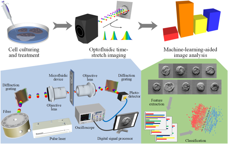
Figure 1
Workflow of the label-free detection of drug-induced morphological variations in cancer cells with optofluidic time-stretch microscopy. The insets show the schematics of optofluidic time-stretch micro...
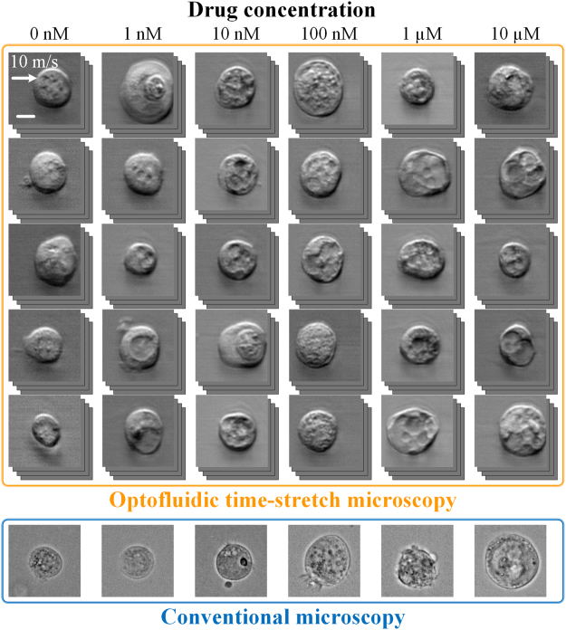
Figure 2
Image libraries of drug-treated and -untreated MCF-7 cells under our optofluidic time-stretch microscope (flowing at a speed of 10u2009m/s). Compared with the static images obtained by a conventional ...
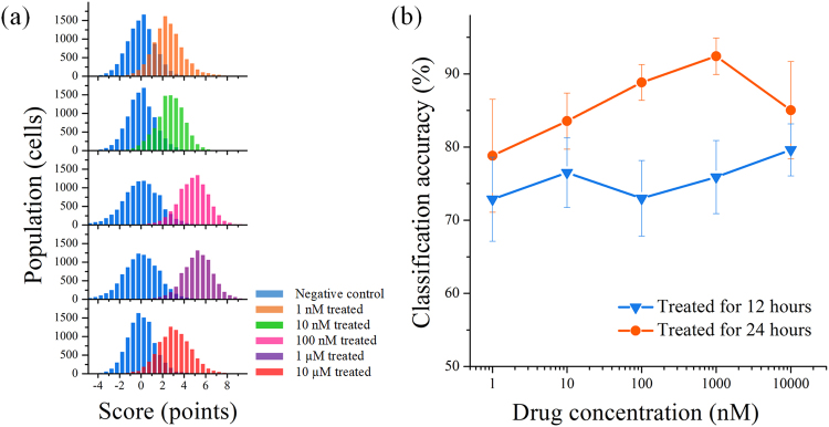
Figure 3
Classification of drug-treated and -untreated cancer cells. ( a ) Histograms of SVM classification scores for MCF-7 cells treated with various concentrations of paclitaxel for 24u2009hours. Each popul...
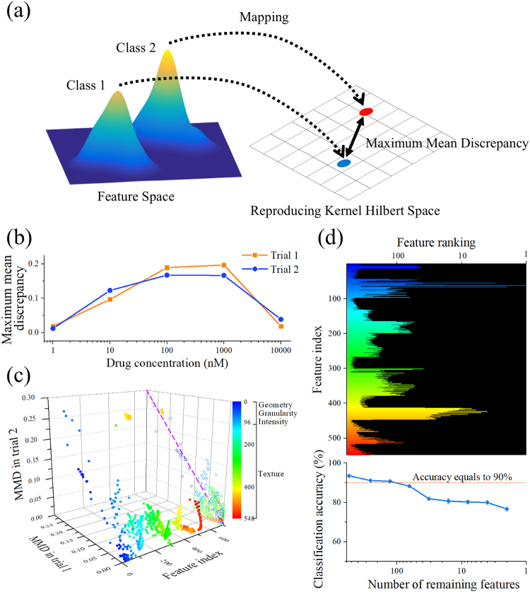
Figure 4
Calculating maximum mean discrepancy (MMD) between the negative control and drug-treated cell population. ( a ) Illustration of the maximum mean discrepancy (MMD). ( b ) MMD between the negative contr...
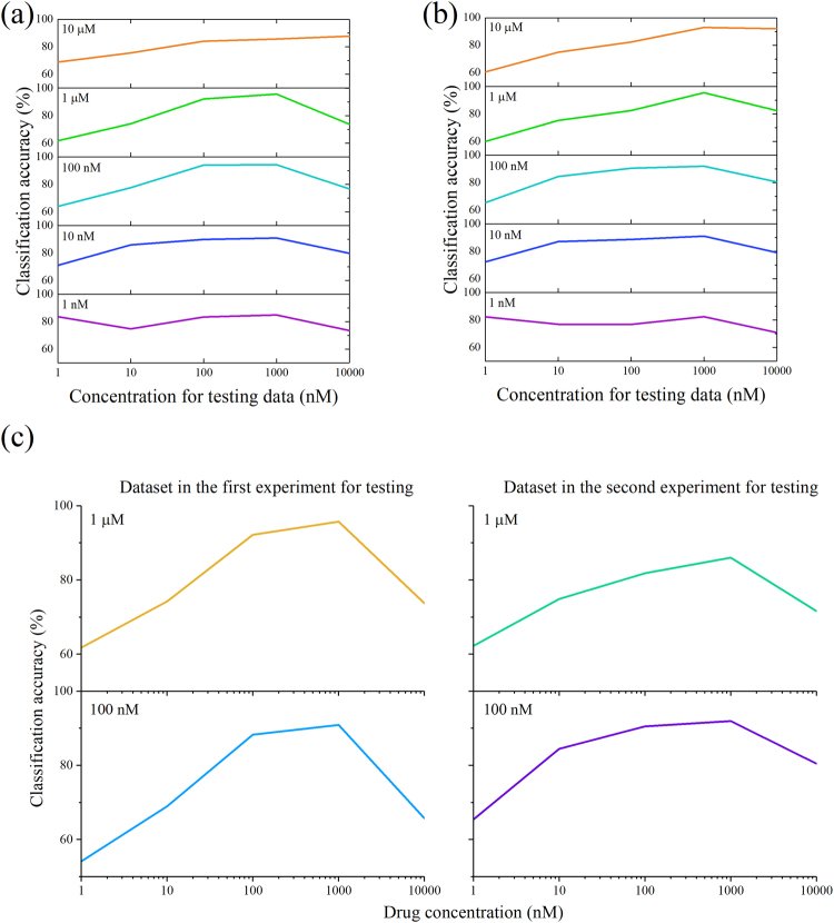
Figure 5
Classification accuracy using single SVM models. Classification accuracy produced by the SVM models in the first experiment ( a ) and the second experiment ( b ). Each row demonstrates the classificat...
Figure images are served from the NIH/NLM PubMed Central Open Access Subset or Europe PMC; copyright remains with the publishers and authors.
💬 Discussion
0 commentsNo comments yet. Be the first to start a discussion!
Leave a Comment