Abstract
AbstractThe mitotic activity index is a key prognostic measure in tumour grading. Microscopy based detection of mitotic nuclei is a significant overhead and necessitates automation. This work proposes deep CNN based multi-phase mitosis detection framework “MP-MitDet” for mitotic nuclei identification in breast cancer histopathological images. The workflow constitutes: (1) label-refiner, (2) tissue-level mitotic region selection, (3) blob analysis, and (4) cell-level refinement. We developed an automatic label-refiner to represent weak labels with semi-sematic information for training of deep CNNs. A deep instance-based detection and segmentation model is used to explore probable mitotic regions on tissue patches. More probable regions are screened based on blob area and then analysed at cell-level by developing a custom CNN classifier “MitosRes-CNN” to filter false mitoses. The performance of the proposed “MitosRes-CNN” is compared with the state-of-the-art CNNs that are adapted to cell-level discrimination through cross-domain transfer learning and by adding task-specific layers. The performance of the proposed framework shows good discrimination ability in terms of F-score (0.75), recall (0.76), precision (0.71) and area under the precision-recall curve (0.78) on challenging TUPAC16 dataset. Promising results suggest good generalization of the proposed framework that can learn characteristic features from heterogenous mitotic nuclei.
🧪 Sample Preparation
🏭 Microscope Brands
🧪 Reagent Suppliers
💻 Software Details
🏛️ Research Organizations (ROR)
Affiliated research institutions:
📋 Methods
This work suggests a multi-phase deep CNN based mitosis detection framework (MP-MitDet) for H&E stained breast cancer histopathological images. The workflow is decomposed into 4 phases: (1) refinement of weakly labelled mitosis dataset, (2) mitotic region selection at tissue-level, (3) blob analysis, and (4) enhancement of mitosis detection results at cell-level. The overall workflow of the proposed detection model is shown in Fig. 2 .
Datasets
TUPAC16 challenge provided a publicly accessible dataset for mitosis detection problem named TUPAC16 auxiliary dataset 21 . This dataset consisted of specified regions of breast biopsies corresponding to 10 HPF selected by the pathologists from WSIs. The provided images were collected from three different centres of Netherlands and were scanned by two different scanners under 40 × magnification. The dataset consisted of 656 images collected from 73 patients. This challenge provided a maximum number of patient samples to date for mitosis detection problem, whereby it provided 50 new patients and included 23 patients’ samples from the AMIDA13 challenge. This dataset is challenging as it provided only centroid labels of the mitoses. Provided mitoses were annotated rigorously by two pathologists. In addition to the TUPAC16 dataset, patient samples from two other previous challenges: MITOS12 and MITOS14 were also included in the training to augment the small number of patient samples and to improve the learning of deep CNN models (details of the dataset are mentioned in Table 1 ) 20 , 22 . All three different datasets were H&E stained and taken from breast tissue biopsies. Table 1 Details of the datasets. Dataset Scanner Resolution (μm/pixel) Spatial Dimension Patients Mitosis TUPAC16 Aperio ScanScope 0.25 2000 × 2000 23 914 Leica SCN400 0.25 5657 × 5657 50 MITOS12 Leica SCN400 0.2456 2084 × 2084 5 226 Hamamatsu 0.2275 2252 × 2250 5 MITOS14 Leica SCN400 0.2456 1539 × 1376 11 749 Hamamatsu 0.2275 1663 × 1485 11 Cross-validation scheme The dataset was divided into train, validation, and test sets, whereas the patient samples in the test were kept the same as mentioned in Wahab et al.’s (2019) 37 study to make the results comparable. Data was divided in such a way that the patient samples were kept disjointed in train, validation, and test to emulate the real-world scenario. The data division is mentioned in Table 2 . Cross validation scheme is kept the same for deep instance based detection and segmentation model employed for tissue level detection as well as for classical and deep classification models used for cell-level classification. All the models were trained with the training dataset and hyperparameters and architectural configurations were selected based on model performance on validation dataset. However, test dataset was kept separate from the training and validation set, and it was used for the final evaluation of the selected models. Table 2 Cross-validation scheme for detection and classification models. Dataset Patient Number Train TUPAC16 patients: 01, 02, 03, 05, 07, 08, 10, 11, 12, 13, 14, 15, 16, 17, 18, 19, 20, 22, 23, 24, 25, 28, 33, 34, 35, 37, 38, 40, 42, 44, 47, 49, 51, 52, 54, 59, 61, 64, 68, 69, 70, 72 All patients from training dataset of MITOS12 and MITOS14 Validation 04, 06, 09, 21, 26, 29, 31, 39, 46, 48, 56, 65, 67, 73 Test 27, 30, 32, 36, 41, 43, 45, 50, 53, 55, 57, 58, 60, 62, 63, 66, 71 Preprocessing and normalization of images Histopathological images were stain normalized initially using Macenko et al.’s 38 technique to mitigate the variations in staining colours. It is expressed in Eq. ( 1 – 3 ). Histopathological images were collected from different pathological laboratories. Each laboratory has its staining protocols, and samples were digitalized using the different scanner, resulting in noise and non-uniformity in colour appearance (shown in Fig. 3 ). All the images were mean normalized and standardized (Eq. 4 ) before assigning them to the machine learning models. 1 documentclass[12pt]{minimal} usepackage{amsmath} usepackage{wasysym} usepackage{amsfonts} usepackage{amssymb} usepackage{amsbsy} usepackage{mathrsfs} usepackage{upgreek} setlength{oddsidemargin}{-69pt} begin{document}$$OD, = , - log_{10} (H)$$end{document} O D = - log 10 ( H ) 2 documentclass[12pt]{minimal} usepackage{amsmath} usepackage{wasysym} usepackage{amsfonts} usepackage{amssymb} usepackage{amsbsy} usepackage{mathrsfs} usepackage{upgreek} setlength{oddsidemargin}{-69pt} begin{document}$$OD, = ,VS$$end{document} O D = V S 3 documentclass[12pt]{minimal} usepackage{amsmath} usepackage{wasysym} usepackage{amsfonts} usepackage{amssymb} usepackage{amsbsy} usepackage{mathrsfs} usepackage{upgreek} setlength{oddsidemargin}{-69pt} begin{document}$$S = V^{ - 1} OD$$end{document} S = V - 1 O D 4 documentclass[12pt]{minimal} usepackage{amsmath} usepackage{wasysym} usepackage{amsfonts} usepackage{amssymb} usepackage{amsbsy} usepackage{mathrsfs} usepackage{upgreek} setlength{oddsidemargin}{-69pt} begin{document}$$H_{norm} = frac{{H_{snorm} - mu }}{sigma }$$end{document} H norm = H snorm - μ σ Figure 3 ( a ) Actual vs. stain normalized images; ( b ) histopathological images from different scanners. In Eq. ( 1 ), documentclass[12pt]{minimal} usepackage{amsmath} usepackage{wasysym} usepackage{amsfonts} usepackage{amssymb} usepackage{amsbsy} usepackage{mathrsfs} usepackage{upgreek} setlength{oddsidemargin}{-69pt} begin{document}$$H$$end{document} H represents histopathological image whose RGB values are transformed to optical density values documentclass[12pt]{minimal} usepackage{amsmath} usepackage{wasysym} usepackage{amsfonts} usepackage{amssymb} usepackage{amsbsy} usepackage{mathrsfs} usepackage{upgreek} setlength{oddsidemargin}{-69pt} begin{document}$$(OD)$$end{document} ( O D ) . Whereas, in Eq. ( 2 ), documentclass[12pt]{minimal} usepackage{amsmath} usepackage{wasysym} usepackage{amsfonts} usepackage{amssymb} usepackage{amsbsy} usepackage{mathrsfs} usepackage{upgreek} setlength{oddsidemargin}{-69pt} begin{document}$$V$$end{document} V represents the stain vectors for H&E, and documentclass[12pt]{minimal} usepackage{amsmath} usepackage{wasysym} usepackage{amsfonts} usepackage{amssymb} usepackage{amsbsy} usepackage{mathrsfs} usepackage{upgreek} setlength{oddsidemargin}{-69pt} begin{document}$$S$$end{document} S shows their saturation value. Equation ( 3 ) is used to express the stain values in a standard quantitative way. In Eq. ( 4 ), documentclass[12pt]{minimal} usepackage{amsmath} usepackage{wasysym} usepackage{amsfonts} usepackage{amssymb} usepackage{amsbsy} usepackage{mathrsfs} usepackage{upgreek} setlength{oddsidemargin}{-69pt} begin{document}$$H_{snorm}$$end{document} H snorm and documentclass[12pt]{minimal} usepackage{amsmath} usepackage{wasysym} usepackage{amsfonts} usepackage{amssymb} usepackage{amsbsy} usepackage{mathrsfs} usepackage{upgreek} setlength{oddsidemargin}{-69pt} begin{document}$$H_{norm}$$end{document} H norm are the stain normalized input and mean-standard deviation normalized pixel values, respectively, whereas documentclass[12pt]{minimal} usepackage{amsmath} usepackage{wasysym} usepackage{amsfonts} usepackage{amssymb} usepackage{amsbsy} usepackage{mathrsfs} usepackage{upgreek} setlength{oddsidemargin}{-69pt} begin{document}$$mu$$end{document} μ and documentclass[12pt]{minimal} usepackage{amsmath} usepackage{wasysym} usepackage{amsfonts} usepackage{amssymb} usepackage{amsbsy} usepackage{mathrsfs} usepackage{upgreek} setlength{oddsidemargin}{-69pt} begin{document}$$sigma$$end{document} σ are used to represent the mean and standard deviation for RGB values of the dataset.
Show full methods section
This work suggests a multi-phase deep CNN based mitosis detection framework (MP-MitDet) for H&E stained breast cancer histopathological images. The workflow is decomposed into 4 phases: (1) refinement of weakly labelled mitosis dataset, (2) mitotic region selection at tissue-level, (3) blob analysis, and (4) enhancement of mitosis detection results at cell-level. The overall workflow of the proposed detection model is shown in Fig. 2 .
Datasets
TUPAC16 challenge provided a publicly accessible dataset for mitosis detection problem named TUPAC16 auxiliary dataset 21 . This dataset consisted of specified regions of breast biopsies corresponding to 10 HPF selected by the pathologists from WSIs. The provided images were collected from three different centres of Netherlands and were scanned by two different scanners under 40 × magnification. The dataset consisted of 656 images collected from 73 patients. This challenge provided a maximum number of patient samples to date for mitosis detection problem, whereby it provided 50 new patients and included 23 patients’ samples from the AMIDA13 challenge. This dataset is challenging as it provided only centroid labels of the mitoses. Provided mitoses were annotated rigorously by two pathologists. In addition to the TUPAC16 dataset, patient samples from two other previous challenges: MITOS12 and MITOS14 were also included in the training to augment the small number of patient samples and to improve the learning of deep CNN models (details of the dataset are mentioned in Table 1 ) 20 , 22 . All three different datasets were H&E stained and taken from breast tissue biopsies. Table 1 Details of the datasets. Dataset Scanner Resolution (μm/pixel) Spatial Dimension Patients Mitosis TUPAC16 Aperio ScanScope 0.25 2000 × 2000 23 914 Leica SCN400 0.25 5657 × 5657 50 MITOS12 Leica SCN400 0.2456 2084 × 2084 5 226 Hamamatsu 0.2275 2252 × 2250 5 MITOS14 Leica SCN400 0.2456 1539 × 1376 11 749 Hamamatsu 0.2275 1663 × 1485 11 Cross-validation scheme The dataset was divided into train, validation, and test sets, whereas the patient samples in the test were kept the same as mentioned in Wahab et al.’s (2019) 37 study to make the results comparable. Data was divided in such a way that the patient samples were kept disjointed in train, validation, and test to emulate the real-world scenario. The data division is mentioned in Table 2 . Cross validation scheme is kept the same for deep instance based detection and segmentation model employed for tissue level detection as well as for classical and deep classification models used for cell-level classification. All the models were trained with the training dataset and hyperparameters and architectural configurations were selected based on model performance on validation dataset. However, test dataset was kept separate from the training and validation set, and it was used for the final evaluation of the selected models. Table 2 Cross-validation scheme for detection and classification models. Dataset Patient Number Train TUPAC16 patients: 01, 02, 03, 05, 07, 08, 10, 11, 12, 13, 14, 15, 16, 17, 18, 19, 20, 22, 23, 24, 25, 28, 33, 34, 35, 37, 38, 40, 42, 44, 47, 49, 51, 52, 54, 59, 61, 64, 68, 69, 70, 72 All patients from training dataset of MITOS12 and MITOS14 Validation 04, 06, 09, 21, 26, 29, 31, 39, 46, 48, 56, 65, 67, 73 Test 27, 30, 32, 36, 41, 43, 45, 50, 53, 55, 57, 58, 60, 62, 63, 66, 71 Preprocessing and normalization of images Histopathological images were stain normalized initially using Macenko et al.’s 38 technique to mitigate the variations in staining colours. It is expressed in Eq. ( 1 – 3 ). Histopathological images were collected from different pathological laboratories. Each laboratory has its staining protocols, and samples were digitalized using the different scanner, resulting in noise and non-uniformity in colour appearance (shown in Fig. 3 ). All the images were mean normalized and standardized (Eq. 4 ) before assigning them to the machine learning models. 1 documentclass[12pt]{minimal} usepackage{amsmath} usepackage{wasysym} usepackage{amsfonts} usepackage{amssymb} usepackage{amsbsy} usepackage{mathrsfs} usepackage{upgreek} setlength{oddsidemargin}{-69pt} begin{document}$$OD, = , - log_{10} (H)$$end{document} O D = - log 10 ( H ) 2 documentclass[12pt]{minimal} usepackage{amsmath} usepackage{wasysym} usepackage{amsfonts} usepackage{amssymb} usepackage{amsbsy} usepackage{mathrsfs} usepackage{upgreek} setlength{oddsidemargin}{-69pt} begin{document}$$OD, = ,VS$$end{document} O D = V S 3 documentclass[12pt]{minimal} usepackage{amsmath} usepackage{wasysym} usepackage{amsfonts} usepackage{amssymb} usepackage{amsbsy} usepackage{mathrsfs} usepackage{upgreek} setlength{oddsidemargin}{-69pt} begin{document}$$S = V^{ - 1} OD$$end{document} S = V - 1 O D 4 documentclass[12pt]{minimal} usepackage{amsmath} usepackage{wasysym} usepackage{amsfonts} usepackage{amssymb} usepackage{amsbsy} usepackage{mathrsfs} usepackage{upgreek} setlength{oddsidemargin}{-69pt} begin{document}$$H_{norm} = frac{{H_{snorm} - mu }}{sigma }$$end{document} H norm = H snorm - μ σ Figure 3 ( a ) Actual vs. stain normalized images; ( b ) histopathological images from different scanners. In Eq. ( 1 ), documentclass[12pt]{minimal} usepackage{amsmath} usepackage{wasysym} usepackage{amsfonts} usepackage{amssymb} usepackage{amsbsy} usepackage{mathrsfs} usepackage{upgreek} setlength{oddsidemargin}{-69pt} begin{document}$$H$$end{document} H represents histopathological image whose RGB values are transformed to optical density values documentclass[12pt]{minimal} usepackage{amsmath} usepackage{wasysym} usepackage{amsfonts} usepackage{amssymb} usepackage{amsbsy} usepackage{mathrsfs} usepackage{upgreek} setlength{oddsidemargin}{-69pt} begin{document}$$(OD)$$end{document} ( O D ) . Whereas, in Eq. ( 2 ), documentclass[12pt]{minimal} usepackage{amsmath} usepackage{wasysym} usepackage{amsfonts} usepackage{amssymb} usepackage{amsbsy} usepackage{mathrsfs} usepackage{upgreek} setlength{oddsidemargin}{-69pt} begin{document}$$V$$end{document} V represents the stain vectors for H&E, and documentclass[12pt]{minimal} usepackage{amsmath} usepackage{wasysym} usepackage{amsfonts} usepackage{amssymb} usepackage{amsbsy} usepackage{mathrsfs} usepackage{upgreek} setlength{oddsidemargin}{-69pt} begin{document}$$S$$end{document} S shows their saturation value. Equation ( 3 ) is used to express the stain values in a standard quantitative way. In Eq. ( 4 ), documentclass[12pt]{minimal} usepackage{amsmath} usepackage{wasysym} usepackage{amsfonts} usepackage{amssymb} usepackage{amsbsy} usepackage{mathrsfs} usepackage{upgreek} setlength{oddsidemargin}{-69pt} begin{document}$$H_{snorm}$$end{document} H snorm and documentclass[12pt]{minimal} usepackage{amsmath} usepackage{wasysym} usepackage{amsfonts} usepackage{amssymb} usepackage{amsbsy} usepackage{mathrsfs} usepackage{upgreek} setlength{oddsidemargin}{-69pt} begin{document}$$H_{norm}$$end{document} H norm are the stain normalized input and mean-standard deviation normalized pixel values, respectively, whereas documentclass[12pt]{minimal} usepackage{amsmath} usepackage{wasysym} usepackage{amsfonts} usepackage{amssymb} usepackage{amsbsy} usepackage{mathrsfs} usepackage{upgreek} setlength{oddsidemargin}{-69pt} begin{document}$$mu$$end{document} μ and documentclass[12pt]{minimal} usepackage{amsmath} usepackage{wasysym} usepackage{amsfonts} usepackage{amssymb} usepackage{amsbsy} usepackage{mathrsfs} usepackage{upgreek} setlength{oddsidemargin}{-69pt} begin{document}$$sigma$$end{document} σ are used to represent the mean and standard deviation for RGB values of the dataset.
Refinement of weakly labelled mitosis dataset
Annotations for the MITOS14 and TUPAC16 datasets are provided as weak labels documentclass[12pt]{minimal} usepackage{amsmath} usepackage{wasysym} usepackage{amsfonts} usepackage{amssymb} usepackage{amsbsy} usepackage{mathrsfs} usepackage{upgreek} setlength{oddsidemargin}{-69pt} begin{document}$$(Y_{centroid} = M_{x,y = c} )$$end{document} ( Y centroid = M x , y = c ) . The labels are represented by centroid pixel ( documentclass[12pt]{minimal} usepackage{amsmath} usepackage{wasysym} usepackage{amsfonts} usepackage{amssymb} usepackage{amsbsy} usepackage{mathrsfs} usepackage{upgreek} setlength{oddsidemargin}{-69pt} begin{document}$$M_{x,y = c}$$end{document} M x , y = c ) of the mitoses, as shown in Fig. 4 b. In practice, it is extremely time-consuming for pathologists to annotate a large number of patient samples manually and assign pixel-level labels. Therefore, an automated labelling approach named as label-refiner is developed to assign the pixel-level labels. Mask R-CNN 39 is used to develop the fine masks for mitoses and it is trained with MITOS12 dataset (Fig. 4 a) having pixel-level annotations documentclass[12pt]{minimal} usepackage{amsmath} usepackage{wasysym} usepackage{amsfonts} usepackage{amssymb} usepackage{amsbsy} usepackage{mathrsfs} usepackage{upgreek} setlength{oddsidemargin}{-69pt} begin{document}$$(Y_{polygon} = M_{x,y = 1}^{s} )$$end{document} ( Y polygon = M x , y = 1 s ) . MITOS12 dataset consists of only 5 patients (Table 1 ), therefore pretrained Mask R-CNN is used and fine-tuned on 338 samples from 5 patients. Strongly labelled dataset helps the Mask R-CNN to learn the morphology of the mitoses. Mask R-CNN architecture is shown in Fig. 5 . The learning stages of Mask R-CNN are divided into (i) Feature Extraction Network (ResNet + Feature Pyramid Network), (ii) Region Proposal Network (RPN), (iii) Region of Interest (ROI) alignment, (iv) Detection and Segmentation. Figure 4 ( a ) Pixel-level annotations; ( b ) weak labels (centroid labels). Figure 5 Architectural details of the Mask R-CNN. The trained Mask R-CNN is used to generate the pixel by pixel masks for the training set (Table 2 ) of mitosis detection module. Generated masks are used as labels for further analysis of the mitosis dataset, whereas segmented blobs that do not correspond to true mitoses are discarded. During the refinement phase, some labels are missed by the detection model for which pseudo labels documentclass[12pt]{minimal} usepackage{amsmath} usepackage{wasysym} usepackage{amsfonts} usepackage{amssymb} usepackage{amsbsy} usepackage{mathrsfs} usepackage{upgreek} setlength{oddsidemargin}{-69pt} begin{document}$$(,Y_{circular} )$$end{document} ( Y circular ) are developed. Pseudo labels documentclass[12pt]{minimal} usepackage{amsmath} usepackage{wasysym} usepackage{amsfonts} usepackage{amssymb} usepackage{amsbsy} usepackage{mathrsfs} usepackage{upgreek} setlength{oddsidemargin}{-69pt} begin{document}$$(,Y_{circular} )$$end{document} ( Y circular ) are generated based on the idea proposed by Li et al. (2019) 15 and represented each mitosis in the form of a circle. Circular annotation is drawn randomly with a radius of 10–16 pixels. So, the developed label-refiner documentclass[12pt]{minimal} usepackage{amsmath} usepackage{wasysym} usepackage{amsfonts} usepackage{amssymb} usepackage{amsbsy} usepackage{mathrsfs} usepackage{upgreek} setlength{oddsidemargin}{-69pt} begin{document}$$f_{refiner} (H_{norm} ,,Y_{centroid} )$$end{document} f refiner ( H norm , Y centroid ) (expressed in Eq. ( 5 )) works by taking input images documentclass[12pt]{minimal} usepackage{amsmath} usepackage{wasysym} usepackage{amsfonts} usepackage{amssymb} usepackage{amsbsy} usepackage{mathrsfs} usepackage{upgreek} setlength{oddsidemargin}{-69pt} begin{document}$$(H_{norm} )$$end{document} ( H norm ) and their weak labels documentclass[12pt]{minimal} usepackage{amsmath} usepackage{wasysym} usepackage{amsfonts} usepackage{amssymb} usepackage{amsbsy} usepackage{mathrsfs} usepackage{upgreek} setlength{oddsidemargin}{-69pt} begin{document}$$(,Y_{centroid} )$$end{document} ( Y centroid ) and returns the semi-semantically labelled dataset documentclass[12pt]{minimal} usepackage{amsmath} usepackage{wasysym} usepackage{amsfonts} usepackage{amssymb} usepackage{amsbsy} usepackage{mathrsfs} usepackage{upgreek} setlength{oddsidemargin}{-69pt} begin{document}$$(Y_{semi - semantic} )$$end{document} ( Y s e m i - s e m a n t i c ) , consisting of true morphology and pseudo representation. The complete workflow of the label refinement phase is shown in Fig. 6 . 5 documentclass[12pt]{minimal} usepackage{amsmath} usepackage{wasysym} usepackage{amsfonts} usepackage{amssymb} usepackage{amsbsy} usepackage{mathrsfs} usepackage{upgreek} setlength{oddsidemargin}{-69pt} begin{document}$$Y_{semi - semantic} = f_{refiner} (H_{norm} ,,Y_{centroid} )$$end{document} Y s e m i - s e m a n t i c = f refiner ( H norm , Y centroid ) Figure 6 Label refinement module (label-refiner) for the weakly annotated dataset. Mitotic region selection at tissue level We exploited multi-objective loss function of Mask R-CNN for mitosis region selection from histopathology tissue patches using weight space TL and hyper-parameter optimization. Workflow of mitotic region selection at tissue-level using multi-objective deep instance based detection and segmentation model is shown Fig. 7 a. The use of multi-objective loss function ( documentclass[12pt]{minimal} usepackage{amsmath} usepackage{wasysym} usepackage{amsfonts} usepackage{amssymb} usepackage{amsbsy} usepackage{mathrsfs} usepackage{upgreek} setlength{oddsidemargin}{-69pt} begin{document}$$L_{multi - obj}$$end{document} L m u l t i - o b j ) expressed in Eq. ( 6 ) helps to improve the mitosis detection task by incorporating the morphology information (Eq. ( 9 )) from segmentation branch along with region information from detection branch that performs bounding box regression and classification (Eq. ( 7 & 8 )). 6 documentclass[12pt]{minimal} usepackage{amsmath} usepackage{wasysym} usepackage{amsfonts} usepackage{amssymb} usepackage{amsbsy} usepackage{mathrsfs} usepackage{upgreek} setlength{oddsidemargin}{-69pt} begin{document}$$L_{multi - obj} = l_{clas} + l_{reg} + l_{mask}$$end{document} L m u l t i - o b j = l clas + l reg + l mask 7 documentclass[12pt]{minimal} usepackage{amsmath} usepackage{wasysym} usepackage{amsfonts} usepackage{amssymb} usepackage{amsbsy} usepackage{mathrsfs} usepackage{upgreek} setlength{oddsidemargin}{-69pt} begin{document}$$l_{clas} = - log P(C_{j}^{*} |C_{j} )$$end{document} l clas = - log P ( C j ∗ | C j ) 8 documentclass[12pt]{minimal} usepackage{amsmath} usepackage{wasysym} usepackage{amsfonts} usepackage{amssymb} usepackage{amsbsy} usepackage{mathrsfs} usepackage{upgreek} setlength{oddsidemargin}{-69pt} begin{document}$$l_{reg} = smooth,L_{1} (B_{j} - B_{j}^{*} )$$end{document} l reg = s m o o t h L 1 ( B j - B j ∗ ) 9 documentclass[12pt]{minimal} usepackage{amsmath} usepackage{wasysym} usepackage{amsfonts} usepackage{amssymb} usepackage{amsbsy} usepackage{mathrsfs} usepackage{upgreek} setlength{oddsidemargin}{-69pt} begin{document}$$l_{mask} (C^{*} ,C) = frac{1}{R times H}sumlimits_{r = 1}^{R} {sumlimits_{c = 1}^{C} {left[ {C_{r,c}^{*} .log C_{r,c} + (1 - C_{r,c}^{*} ).log (1 - C_{r,c} )} right]} }$$end{document} l mask ( C ∗ , C ) = 1 R × H ∑ r = 1 R ∑ c = 1 C C r , c ∗ . log C r , c + ( 1 - C r , c ∗ ) . log ( 1 - C r , c ) Figure 7 Work flow diagram, ( a ) mitotic region selection at tissue-level using multi-objective deep instance based detection and segmentation model, ( b ) blob analysis, ( c ), enhancement using cell-level classification. Equation ( 7 & 8 ) represent the classification documentclass[12pt]{minimal} usepackage{amsmath} usepackage{wasysym} usepackage{amsfonts} usepackage{amssymb} usepackage{amsbsy} usepackage{mathrsfs} usepackage{upgreek} setlength{oddsidemargin}{-69pt} begin{document}$$(l_{clas} )$$end{document} ( l clas ) , and box regression documentclass[12pt]{minimal} usepackage{amsmath} usepackage{wasysym} usepackage{amsfonts} usepackage{amssymb} usepackage{amsbsy} usepackage{mathrsfs} usepackage{upgreek} setlength{oddsidemargin}{-69pt} begin{document}$$(l_{reg} )$$end{document} ( l reg ) loss, respectively, whereas documentclass[12pt]{minimal} usepackage{amsmath} usepackage{wasysym} usepackage{amsfonts} usepackage{amssymb} usepackage{amsbsy} usepackage{mathrsfs} usepackage{upgreek} setlength{oddsidemargin}{-69pt} begin{document}$$C_{j}$$end{document} C j and documentclass[12pt]{minimal} usepackage{amsmath} usepackage{wasysym} usepackage{amsfonts} usepackage{amssymb} usepackage{amsbsy} usepackage{mathrsfs} usepackage{upgreek} setlength{oddsidemargin}{-69pt} begin{document}$$B_{j}$$end{document} B j denote the predicted class label and estimated bounding box coordinates, respectively, for j th anchor. Likewise, documentclass[12pt]{minimal} usepackage{amsmath} usepackage{wasysym} usepackage{amsfonts} usepackage{amssymb} usepackage{amsbsy} usepackage{mathrsfs} usepackage{upgreek} setlength{oddsidemargin}{-69pt} begin{document}$$C_{j}^{*}$$end{document} C j ∗ and documentclass[12pt]{minimal} usepackage{amsmath} usepackage{wasysym} usepackage{amsfonts} usepackage{amssymb} usepackage{amsbsy} usepackage{mathrsfs} usepackage{upgreek} setlength{oddsidemargin}{-69pt} begin{document}$$B_{j}^{*}$$end{document} B j ∗ are used to represent the ground-truth values for j th anchor. Bounding box regression branch returns the real values therefore the difference between ground-truth spatial coordinates and predicted coordinates is minimized by computing smooth L1 loss (Eq. ( 8 )). The segmentation loss function documentclass[12pt]{minimal} usepackage{amsmath} usepackage{wasysym} usepackage{amsfonts} usepackage{amssymb} usepackage{amsbsy} usepackage{mathrsfs} usepackage{upgreek} setlength{oddsidemargin}{-69pt} begin{document}$$(l_{mask} )$$end{document} ( l mask ) is estimated by using Eq. ( 9 ), whereas spatial dimensions of the input region proposal are represented via documentclass[12pt]{minimal} usepackage{amsmath} usepackage{wasysym} usepackage{amsfonts} usepackage{amssymb} usepackage{amsbsy} usepackage{mathrsfs} usepackage{upgreek} setlength{oddsidemargin}{-69pt} begin{document}$$(R times H)$$end{document} ( R × H ) . In this equation, documentclass[12pt]{minimal} usepackage{amsmath} usepackage{wasysym} usepackage{amsfonts} usepackage{amssymb} usepackage{amsbsy} usepackage{mathrsfs} usepackage{upgreek} setlength{oddsidemargin}{-69pt} begin{document}$$(.)$$end{document} ( . ) operator denotes the multiplication sign, whereas documentclass[12pt]{minimal} usepackage{amsmath} usepackage{wasysym} usepackage{amsfonts} usepackage{amssymb} usepackage{amsbsy} usepackage{mathrsfs} usepackage{upgreek} setlength{oddsidemargin}{-69pt} begin{document}$$C_{r,c}^{*}$$end{document} C r , c ∗ indicates the ground-truth class for documentclass[12pt]{minimal} usepackage{amsmath} usepackage{wasysym} usepackage{amsfonts} usepackage{amssymb} usepackage{amsbsy} usepackage{mathrsfs} usepackage{upgreek} setlength{oddsidemargin}{-69pt} begin{document}$$(r,c)$$end{document} ( r , c ) coordinates and documentclass[12pt]{minimal} usepackage{amsmath} usepackage{wasysym} usepackage{amsfonts} usepackage{amssymb} usepackage{amsbsy} usepackage{mathrsfs} usepackage{upgreek} setlength{oddsidemargin}{-69pt} begin{document}$$C_{r,c}$$end{document} C r , c shows predicted class probability at documentclass[12pt]{minimal} usepackage{amsmath} usepackage{wasysym} usepackage{amsfonts} usepackage{amssymb} usepackage{amsbsy} usepackage{mathrsfs} usepackage{upgreek} setlength{oddsidemargin}{-69pt} begin{document}$$(r,c)$$end{document} ( r , c ) coordinates of the image. In this study, mitotic region selection is considered as a binary class detection problem. For the training of detection module (Mask R-CNN), histopathological images are labelled in a COCO format 40 by defining mitosis as an object of interest, whereas all other cellular/nuclear components and stroma are labelled as background. The backbone of Mask R-CNN was built on Feature Pyramid Network based ResNet101 34 , 41 shown in Figs. 5 and 7 for the learning of enriched deep feature hierarchies. The advantage of using this network is that it learns strong semantic information while retaining spatial information at different scales. Mitoses are small in size and are expressed via few pixels in the later layers of deep architecture however, this information is not enough for object detection.
Feature Pyramid Network
(FPN) alleviates this problem by extracting the feature representation of the object at different scales 41 . Feature representation learned from FPN is assigned to the RPN to extract the probable regions. In RPN, region proposals are searched by using 12 anchors by setting aspect ratios as {1:2, 1:1, 2:1} on four different scales {32 × 32, 64 × 64, 128 × 128, 256 × 256}. RPN selects the region proposals by computing Intersection over Union (IoU) of each region proposal with ground truth and retains only those regions that overlap by at least 70%. These region proposals are mapped to the feature map using ROI align that resizes them using bi-linear interpolation and assigns them to the detection and segmentation head for the classification of the selected regions. Training of detection model using weight space transfer learning Mask R-CNN is trained on 3904 images of train dataset (Table 2 ) by exploiting the idea of weight transfer of pre-trained architecture to adapt the deep architecture on a small mitosis dataset consisting of 61 patients 42 . Deep NNs usually require a massive amount of data for training and suffer from overfitting on insufficient data. TL addresses this problem by allowing to reuse the knowledge of the pre-trained network to a new task and has shown remarkable results when labelled data is insufficient in the target domain. TL can be employed by using pre-trained architecture as a fixed feature extractor, freezing lower layers and fine-tuning higher layers, or leveraging parameter space of pre-trained architecture to the target domain 43 . In this work, the backbone architecture of Mask R-CNN is pre-trained on 1 million natural images from ImageNet, whereas the detection and segmentation head is pre-trained on the COCO dataset 40 , 44 . So, we define the source domain as documentclass[12pt]{minimal} usepackage{amsmath} usepackage{wasysym} usepackage{amsfonts} usepackage{amssymb} usepackage{amsbsy} usepackage{mathrsfs} usepackage{upgreek} setlength{oddsidemargin}{-69pt} begin{document}$$D(S) = left{ {I_{N} ,P(I_{N} )} right}$$end{document} D ( S ) = I N , P ( I N ) where documentclass[12pt]{minimal} usepackage{amsmath} usepackage{wasysym} usepackage{amsfonts} usepackage{amssymb} usepackage{amsbsy} usepackage{mathrsfs} usepackage{upgreek} setlength{oddsidemargin}{-69pt} begin{document}$$I_{N}$$end{document} I N represents the natural images and documentclass[12pt]{minimal} usepackage{amsmath} usepackage{wasysym} usepackage{amsfonts} usepackage{amssymb} usepackage{amsbsy} usepackage{mathrsfs} usepackage{upgreek} setlength{oddsidemargin}{-69pt} begin{document}$$P(I_{N} )$$end{document} P ( I N ) represents its marginal distribution. The knowledge domain of a pre-trained network documentclass[12pt]{minimal} usepackage{amsmath} usepackage{wasysym} usepackage{amsfonts} usepackage{amssymb} usepackage{amsbsy} usepackage{mathrsfs} usepackage{upgreek} setlength{oddsidemargin}{-69pt} begin{document}$$N_{S} = f_{S} (theta_{S} ,left{ {I_{N} ,Y_{N} } right})$$end{document} N S = f S ( θ S , I N , Y N ) constitutes the images documentclass[12pt]{minimal} usepackage{amsmath} usepackage{wasysym} usepackage{amsfonts} usepackage{amssymb} usepackage{amsbsy} usepackage{mathrsfs} usepackage{upgreek} setlength{oddsidemargin}{-69pt} begin{document}$$(I_{N} )$$end{document} ( I N ) , labels documentclass[12pt]{minimal} usepackage{amsmath} usepackage{wasysym} usepackage{amsfonts} usepackage{amssymb} usepackage{amsbsy} usepackage{mathrsfs} usepackage{upgreek} setlength{oddsidemargin}{-69pt} begin{document}$$(Y_{N} )$$end{document} ( Y N ) , and parameter space documentclass[12pt]{minimal} usepackage{amsmath} usepackage{wasysym} usepackage{amsfonts} usepackage{amssymb} usepackage{amsbsy} usepackage{mathrsfs} usepackage{upgreek} setlength{oddsidemargin}{-69pt} begin{document}$$(theta_{S} )$$end{document} ( θ S ) . During training, we adapted the parameter space documentclass[12pt]{minimal} usepackage{amsmath} usepackage{wasysym} usepackage{amsfonts} usepackage{amssymb} usepackage{amsbsy} usepackage{mathrsfs} usepackage{upgreek} setlength{oddsidemargin}{-69pt} begin{document}$$(theta_{S} )$$end{document} ( θ S ) by finetuning the network end to end by assigning histopathological images documentclass[12pt]{minimal} usepackage{amsmath} usepackage{wasysym} usepackage{amsfonts} usepackage{amssymb} usepackage{amsbsy} usepackage{mathrsfs} usepackage{upgreek} setlength{oddsidemargin}{-69pt} begin{document}$$(I_{H} )$$end{document} ( I H ) from the target domain documentclass[12pt]{minimal} usepackage{amsmath} usepackage{wasysym} usepackage{amsfonts} usepackage{amssymb} usepackage{amsbsy} usepackage{mathrsfs} usepackage{upgreek} setlength{oddsidemargin}{-69pt} begin{document}$$D(T) = left{ {I_{H} ,P(I_{H} )} right}$$end{document} D ( T ) = I H , P ( I H ) . This finetuned architecture is defined by documentclass[12pt]{minimal} usepackage{amsmath} usepackage{wasysym} usepackage{amsfonts} usepackage{amssymb} usepackage{amsbsy} usepackage{mathrsfs} usepackage{upgreek} setlength{oddsidemargin}{-69pt} begin{document}$$N_{T} = f_{T} (theta_{T} ,left{ {I_{H} ,Y_{H} } right})$$end{document} N T = f T ( θ T , I H , Y H ) and is used for mitotic region selection.
Blob analysis
In this phase, Mask R-CNN predictions are filtered out at threshold cut-off of 0.5 and all regions that are predicted with more than 50% confidence as mitotic regions are regressed to patient’s tissue patches (Fig. 7 b). Candidate mitotic nuclei that are selected are considered as blobs. On the selected regions, blob analysis is performed to retain blobs with an area more than 600 pixels and fragmentary blobs are removed. Bounding boxes for training dataset are analysed and the false positives are separated from the true positives based on their centroid distance from ground truth (Fig. 7 c). Predicted bounding boxes that do not lie within the 30-pixel distance of ground truth are considered as false positives, whereas other predictions are kept as true mitosis. Enhancement of mitosis detection results at cell-level In the last phase, refinement of the selected mitotic regions is performed to reduce the false positives (Fig. 7 c). Therefore, custom made deep CNN “MitosRes-CNN” is proposed for the analysis of selected cells to discriminate hard negative examples from true mitoses. Network topology including depth and width are selected based on validation dataset. The performance of the proposed architecture is compared with the state-of-the-art deep CNN architectures and classical machine learning models. Details of this section are mentioned below. Augmentation and oversampling of the mitotic nuclei Histopathological images exhibit colour appearance multiplicity due to variation in staining protocols across labs and image acquisition under different scanners. Different image variations are applied on-the-fly during the classifier’s training to make it robust towards unseen patient examples. Augmentation strategies include horizontal and vertical flip, rotation, and colour jitters. Mitotic examples are augmented by extracting patches at various positions to avoid the overfitting. Furthermore, during training, the effect of imbalance is reduced by controlling the proportion of minority and majority class by fetching more positive examples based on the ratio of negative and positive examples. Validation and test sets are drawn from patients without augmentation to emulate the real-world scenarios.
Proposed MitosRes-CNN for mitosis classification
In this work, we proposed a new custom CNN “MitosRes-CNN” for the discrimination of false positives from the true mitotic nuclei. The proposed architectural scheme is shown in Fig. 8 . The proposed MitosRes-CNN is formulated of three custom residual blocks with shortcut links. Residual learning 34 [Eq. ( 10 – 12 )] is implemented to tackle the problem of vanishing gradient. Moreover, it performs reference-based optimization of weights by comparing transformed feature-maps with input feature-maps, [as shown in Eq. ( 10 – 12 )] thus it encourages each block to learn useful features. Figure 8 Block diagram of the proposed MitosRes-CNN. Within each custom residual block, set of transformations are implemented to better approximate the data representation, whereas the concept of the effective receptive field 45 is exploited by convolving the feature-maps with the same size of filters. The transformations are comprised of 3 × 3 convolution operation (Eq. ( 10 )) in combination with batch normalization to smoothen the gradient-based learning 46 . Leaky ReLU (Eq. ( 12 )) is used as a activation function to incorporate the non-linearity and to add the sparsity 47 . Leaky ReLU addresses the problem of dead neurons by permitting the positive activation ( documentclass[12pt]{minimal} usepackage{amsmath} usepackage{wasysym} usepackage{amsfonts} usepackage{amssymb} usepackage{amsbsy} usepackage{mathrsfs} usepackage{upgreek} setlength{oddsidemargin}{-69pt} begin{document}$$a,$$end{document} a ) values as such, whereby assigning a small gradient to negative activations ( documentclass[12pt]{minimal} usepackage{amsmath} usepackage{wasysym} usepackage{amsfonts} usepackage{amssymb} usepackage{amsbsy} usepackage{mathrsfs} usepackage{upgreek} setlength{oddsidemargin}{-69pt} begin{document}$$a,$$end{document} a ). 10 documentclass[12pt]{minimal} usepackage{amsmath} usepackage{wasysym} usepackage{amsfonts} usepackage{amssymb} usepackage{amsbsy} usepackage{mathrsfs} usepackage{upgreek} setlength{oddsidemargin}{-69pt} begin{document}$$O_{x,y}^{l + 1} = sumlimits_{c}^{C} {sumlimits_{p,q}^{P,Q} {k_{i,j} ,M_{p + i,q + j}^{l} } } + b$$end{document} O x , y l + 1 = ∑ c C ∑ p , q P , Q k i , j M p + i , q + j l + b 11 documentclass[12pt]{minimal} usepackage{amsmath} usepackage{wasysym} usepackage{amsfonts} usepackage{amssymb} usepackage{amsbsy} usepackage{mathrsfs} usepackage{upgreek} setlength{oddsidemargin}{-69pt} begin{document}$$M_{x,y}^{l + 1} = O_{x,y}^{l + 1} + M_{x,y}^{l}$$end{document} M x , y l + 1 = O x , y l + 1 + M x , y l 12 documentclass[12pt]{minimal} usepackage{amsmath} usepackage{wasysym} usepackage{amsfonts} usepackage{amssymb} usepackage{amsbsy} usepackage{mathrsfs} usepackage{upgreek} setlength{oddsidemargin}{-69pt} begin{document}$$M_{x,y}^{l} = M_{x,y}^{l + 1} - O_{x,y}^{l + 1}$$end{document} M x , y l = M x , y l + 1 - O x , y l + 1 13 documentclass[12pt]{minimal} usepackage{amsmath} usepackage{wasysym} usepackage{amsfonts} usepackage{amssymb} usepackage{amsbsy} usepackage{mathrsfs} usepackage{upgreek} setlength{oddsidemargin}{-69pt} begin{document}$$f(a) = left{ {begin{array}{*{20}l} a hfill & {if,a, > ,0} hfill \ {0.01a} hfill & {otherwise} hfill \ end{array} } right}$$end{document} f ( a ) = a i f a > 0 0.01 a otherwise Equation ( 10 ) expresses convolution operation performed by convolution layer, whereas documentclass[12pt]{minimal} usepackage{amsmath} usepackage{wasysym} usepackage{amsfonts} usepackage{amssymb} usepackage{amsbsy} usepackage{mathrsfs} usepackage{upgreek} setlength{oddsidemargin}{-69pt} begin{document}$$M_{p,q}^{l}$$end{document} M p , q l represents the input feature map of spatial size documentclass[12pt]{minimal} usepackage{amsmath} usepackage{wasysym} usepackage{amsfonts} usepackage{amssymb} usepackage{amsbsy} usepackage{mathrsfs} usepackage{upgreek} setlength{oddsidemargin}{-69pt} begin{document}$$(P times Q,{text{pixels}}),$$end{document} ( P × Q pixels ) for documentclass[12pt]{minimal} usepackage{amsmath} usepackage{wasysym} usepackage{amsfonts} usepackage{amssymb} usepackage{amsbsy} usepackage{mathrsfs} usepackage{upgreek} setlength{oddsidemargin}{-69pt} begin{document}$$l{text{th}}$$end{document} l th layer, documentclass[12pt]{minimal} usepackage{amsmath} usepackage{wasysym} usepackage{amsfonts} usepackage{amssymb} usepackage{amsbsy} usepackage{mathrsfs} usepackage{upgreek} setlength{oddsidemargin}{-69pt} begin{document}$$k$$end{document} k denotes the kth convolution kernel and b is for bias. Whereas, c shows the feature map depth, ( i, j ) represents spatial coordinates of kernel and ( p + i, q + j ) shows the receptive field occupied by kernel. In Eq. ( 11 ), documentclass[12pt]{minimal} usepackage{amsmath} usepackage{wasysym} usepackage{amsfonts} usepackage{amssymb} usepackage{amsbsy} usepackage{mathrsfs} usepackage{upgreek} setlength{oddsidemargin}{-69pt} begin{document}$$M_{x,y}^{l}$$end{document} M x , y l is the input assigned to residual block, whereas documentclass[12pt]{minimal} usepackage{amsmath} usepackage{wasysym} usepackage{amsfonts} usepackage{amssymb} usepackage{amsbsy} usepackage{mathrsfs} usepackage{upgreek} setlength{oddsidemargin}{-69pt} begin{document}$$O_{x,y}^{l + 1}$$end{document} O x , y l + 1 is a transformed (convolved) feature-map that is output from documentclass[12pt]{minimal} usepackage{amsmath} usepackage{wasysym} usepackage{amsfonts} usepackage{amssymb} usepackage{amsbsy} usepackage{mathrsfs} usepackage{upgreek} setlength{oddsidemargin}{-69pt} begin{document}$$l{text{th}}$$end{document} l th layer. Equation ( 12 ) shows the residual output ( documentclass[12pt]{minimal} usepackage{amsmath} usepackage{wasysym} usepackage{amsfonts} usepackage{amssymb} usepackage{amsbsy} usepackage{mathrsfs} usepackage{upgreek} setlength{oddsidemargin}{-69pt} begin{document}$$M_{x,y}^{l + 1} - O_{x,y}^{l + 1}$$end{document} M x , y l + 1 - O x , y l + 1 ). 14 documentclass[12pt]{minimal} usepackage{amsmath} usepackage{wasysym} usepackage{amsfonts} usepackage{amssymb} usepackage{amsbsy} usepackage{mathrsfs} usepackage{upgreek} setlength{oddsidemargin}{-69pt} begin{document}$$A_{x,y}^{l + 1} = f_{avg} (M_{x,y}^{l + 1} )$$end{document} A x , y l + 1 = f avg ( M x , y l + 1 ) At the end of each residual block, downsampling of the feature-map is performed using average pooling (Eq. ( 14 )) to incorporate both low and high-level responses. In Eq. ( 14 ) average pooling operation is denoted via documentclass[12pt]{minimal} usepackage{amsmath} usepackage{wasysym} usepackage{amsfonts} usepackage{amssymb} usepackage{amsbsy} usepackage{mathrsfs} usepackage{upgreek} setlength{oddsidemargin}{-69pt} begin{document}$$f_{avg} (.)$$end{document} f avg ( . ) and documentclass[12pt]{minimal} usepackage{amsmath} usepackage{wasysym} usepackage{amsfonts} usepackage{amssymb} usepackage{amsbsy} usepackage{mathrsfs} usepackage{upgreek} setlength{oddsidemargin}{-69pt} begin{document}$$A_{x,y}^{l + 1}$$end{document} A x , y l + 1 represents its outputs for l th layer. Pooling operation helps in reducing the overfitting and to learn the invariant features. Average pooling operation is followed by a 1 × 1 convolution to increase the number of feature-maps 9 . The number of feature-maps is increased three times at the end of each block. Each block assigns its output to the next block in a feed-forward manner as well as connected via shortcut link (Eq. ( 11 & 12 )) to provide direct access to the gradient. Dropout with a 50% probability is used for fully connected layers to limit the overfitting. SoftMax is used at the end of a fully connected layer to compute the probability of each sample belonging to mitosis or non-mitosis. Details of the proposed architecture are mentioned in Table 3 . Weights (W) of the proposed network are initialized using Glorot uniform random weight initialization strategy (Eq. ( 15 )) and bias (b) is initialized with 0. 15 documentclass[12pt]{minimal} usepackage{amsmath} usepackage{wasysym} usepackage{amsfonts} usepackage{amssymb} usepackage{amsbsy} usepackage{mathrsfs} usepackage{upgreek} setlength{oddsidemargin}{-69pt} begin{document}$$Wsim Uleft[ { - frac{1}{z},frac{1}{z}} right],,,Uleft[ { - n,n} right]$$end{document} W ∼ U - 1 z , 1 z , U - n , n Table 3 Architectural details of the proposed MitosRes-CNN. Layer number Processing unit Input Output Filters Filter size Stride Zero padding Input layer Conv2D + BatchNorm2D + Leaky ReLU 3 × 120 × 120 32 × 60 × 60 32 3 × 3 2 1 Block 1 Conv2D + BatchNorm2D 32 × 60 × 60 64 × 60 × 60 64 1 × 1 1 1 Conv2D + BatchNorm2D [[64 × 60 × 60] × 3 + Leaky ReLU] × 3 64 × 60 × 60 64 3 × 3 1 1 AvgPool2D 64 × 60 × 60 64 × 30 × 30 64 3 × 3 2 1 Conv2D + BatchNorm2D + Leaky ReLU 64 × 30 × 30 96 × 30 × 30 96 1 × 1 1 0 Block 1 skip connection Conv2D + BatchNorm2D 32 × 60 × 60 96 × 30x × 30 96 1 × 1 2 0 Block 2 Conv2D + BatchNorm2D [[96 × 30 × 30] × 3 + Leaky ReLU] × 3 96 × 30 × 30 96 3 × 3 1 1 AvgPool2D 96 × 30 × 30 96 × 15 × 15 96 3 × 3 2 1 Conv2D + BatchNorm2D + Leaky ReLU 96 × 15 × 15 288 × 15 × 15 96 1 × 1 1 0 Block 2 skip connection Conv2D + BatchNorm2D 96 × 30 × 30 288 × 15 × 15 288 1 × 1 2 0 Block 3 Conv2D + BatchNorm2D [[288 × 15 × 15] × 3 + Leaky ReLU] × 2 288 × 15 × 15 288 3 × 3 1 1 Conv2D + BatchNorm2D [288 × 15 × 15] × 2 + Leaky ReLU 288 × 15 × 15 288 3 × 3 1 1 AvgPool2D 288 × 15 × 15 288 × 7 × 7 288 3 × 3 2 1 Conv2D + BatchNorm2D + Leaky ReLU 288 × 7 × 7 512 × 7 × 7 512 3 × 3 1 1 Block 3 skip connection Conv2D + BatchNorm2D 288 × 15 × 15 512 × 7 × 7 512 1 × 1 2 0 Average pooling AdaptiveAvgPool2D (4 × 4) Dropout ( p = 0.5) Dense Fully Connected 8192 150 150 1 – – Dropout ( p = 0.5) Batch normalization Batch normalization 1D Dense Fully Connected 150 2 2 1 – – Softmax In the above Eq. ( 15 ), W specifies the weight vector of network, U represents the uniform distribution that is drawn from range (-n, n) and z is the size of the previous layer. Cross-domain adaptation of deep CNNs for mitosis classification Deep CNNs have shown exemplary performance in diverse image classification tasks 9 . Deep networks learn features in a hierarchical manner, including generic and high-level features specific to the problem. This distinct characteristic allows us to reuse the pre-trained architectures for diverse tasks. Domain adaptation is a type of TL that allows reusing the already pre-trained architecture to a new problem. In this special type of TL, both target and source domains belong to different data distribution but are assigned to the same task. The advantage of this TL is gaining many low and intermediate level features that are shared among the diverse categories of images. In this study, we have exploited the concept of supervised cross-domain feature space adaptation and leveraged the knowledge of state-of-the-art deep CNNs models that are pre-trained on the ImageNet dataset for mitosis recognition problem. In this case, source documentclass[12pt]{minimal} usepackage{amsmath} usepackage{wasysym} usepackage{amsfonts} usepackage{amssymb} usepackage{amsbsy} usepackage{mathrsfs} usepackage{upgreek} setlength{oddsidemargin}{-69pt} begin{document}$$D(S) = { I_{N} ,P(I_{N} )}$$end{document} D ( S ) = { I N , P ( I N ) } and target documentclass[12pt]{minimal} usepackage{amsmath} usepackage{wasysym} usepackage{amsfonts} usepackage{amssymb} usepackage{amsbsy} usepackage{mathrsfs} usepackage{upgreek} setlength{oddsidemargin}{-69pt} begin{document}$$D(T) = { I_{H} ,P(I_{H} )}$$end{document} D ( T ) = { I H , P ( I H ) } domains share the low and intermediate level features ( documentclass[12pt]{minimal} usepackage{amsmath} usepackage{wasysym} usepackage{amsfonts} usepackage{amssymb} usepackage{amsbsy} usepackage{mathrsfs} usepackage{upgreek} setlength{oddsidemargin}{-69pt} begin{document}$$I_{N} = I_{H}$$end{document} I N = I H ) and both are assigned to the classification task but they follow different marginal distribution documentclass[12pt]{minimal} usepackage{amsmath} usepackage{wasysym} usepackage{amsfonts} usepackage{amssymb} usepackage{amsbsy} usepackage{mathrsfs} usepackage{upgreek} setlength{oddsidemargin}{-69pt} begin{document}$$P(I_{N} ) ne P(I_{H} )$$end{document} P ( I N ) ≠ P ( I H ) . Well-known deep CNN models: VGG, ResNet, DenseNet, ResNext, SENet and PolyNet with diverse architectural designs are modified by keeping feature extraction layers as such and adding average pooling layer in alliance with additional fully connected layers to align the network towards the mitosis specific features (shown in Fig. 9 ). The number of filters in task specific fully connected layers and filter size for adaptive average pooling are set based on the validation dataset (Table 2 ). Details of the architectures are mentioned in Table 4 . The entire network is fine-tuned via the back-propagation algorithm on the mitosis dataset to obtain target domain specific semantically meaningful features. Figure 9 Cross-domain TL of the state-of-the-art CNN architectures. Table 4 Cross domain adaptation of the state-of-the-art CNNs. CNN backbone Adaptive average pooling Fully connect layers SE-ResNet50 4 × 4 [4 × 4 × 2048, 950] [950, 2] PolyNet-152 1 × 1 [2048, 2] ResNext50 4 × 4 [4 × 4 × 2048, 750] [750, 2] DenseNet201 7 × 7 [7 × 7 × 1920, 750] [750, 2] VGG16 4 × 4 [4 × 4 × 512, 750] [750, 2] ResNet18 4 × 4 [4 × 4 × 512, 750] [750, 2] Mitosis classification using classical classifiers Classical classification algorithms, including Naive Bayes, Logistic regression, SVM, Decision tree, Random Forest, and XGBoost, are also evaluated for mitosis detection problem. These classifiers were trained on the original feature space as well as on the HOG and LBP extracted feature space.
Performance metrics
The performance of the proposed Mitosis detection framework is evaluated using F-score, Recall, Precision, and Precision-Recall (PR) curve (Eqs. 16 – 18 ). Mitosis detection is a class imbalance problem, where under-representation of mitoses biases the performance measure that assigns equal weightage to each class. F-score evaluates the classifier’s correctness by computing the weighted average of precision and recall (Eq. 18 ). A recall is computed based on the criterion specified for automated mitosis detection modules 48 . According to it, mitosis in the telophase phase is under duplication; therefore, it is counted once, and all the mitoses that lie within 30 pixels of ground truth are counted as true mitoses. 16 documentclass[12pt]{minimal} usepackage{amsmath} usepackage{wasysym} usepackage{amsfonts} usepackage{amssymb} usepackage{amsbsy} usepackage{mathrsfs} usepackage{upgreek} setlength{oddsidemargin}{-69pt} begin{document}$${text{Recall }}=frac{{{text{Truely}},{text{Predicted}},{text{Mitoses}}}}{{{text{Total}},{text{Mitoses}}}}$$end{document} Recall = Truely Predicted Mitoses Total Mitoses 17 documentclass[12pt]{minimal} usepackage{amsmath} usepackage{wasysym} usepackage{amsfonts} usepackage{amssymb} usepackage{amsbsy} usepackage{mathrsfs} usepackage{upgreek} setlength{oddsidemargin}{-69pt} begin{document}$${text{Precision }}=frac{{{text{Truely}},{text{Predicted}},{text{Mitoses}}}}{{{text{Truely}},{text{Predicted}},{text{Mitoses}},{ + },{text{Falsely}},{text{Predicted}},{text{Mitoses}}}}$$end{document} Precision = Truely Predicted Mitoses Truely Predicted Mitoses + Falsely Predicted Mitoses 18 documentclass[12pt]{minimal} usepackage{amsmath} usepackage{wasysym} usepackage{amsfonts} usepackage{amssymb} usepackage{amsbsy} usepackage{mathrsfs} usepackage{upgreek} setlength{oddsidemargin}{-69pt} begin{document}$${text{F {-} Score }}= 2 times frac{{{{{rm Recall} times {rm Precison}}}}}{{{{rm Recall} + {rm Precison}}}}$$end{document} F - Score = 2 × Recall × Precison Recall + Precison In the above equation, recall suggests the detection rate, whereas precision shows the closeness of the predicted classes to the ground truth.
Data preparation for detection and classification models
Patches of size 512 × 512 pixels with 15% overlap were extracted for label refinement and mitosis detection at tissue-level stage for the training of Mask R-CNN. Whereas patches of 80 × 80 pixels were generated for the training of classification models. Input images for classification were resized to 120 × 120 and 224 × 224 pixels for custom and state-of-the-art CNN, respectively, using bilinear interpolation.
Parameter settings
Custom and pre-trained CNN architectures were fine-tuned using cross-entropy loss function by setting batch size equal to 16 and 6, respectively, assigning a learning rate of 1e−3, and weight decay of 1e−5 for 250 epochs. During training the model with best weight state was saved based on the validation dataset. Mask R-CNN was trained for 30,000 epochs using batch size 2, and the learning rate equal to 0.00025. The number of region proposals was set to be 128 for assigning mitosis and non-mitosis examples to ROI head for classification. Mask R-CNN and classification based CNN were optimized using SGD with warmuprestart and cosine annealing optimization strategy, respectively.
📊 Figures
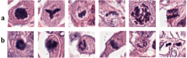
Figure 1
Histopathology patches from TUPAC16 dataset showing heterogeneity in mitosis appearance and their close similarity with non-mitosis, panels ( a , b ) showing mitotic and non-mitotic nuclei, respective...
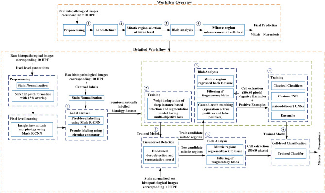
Figure 2
Complete workflow of the proposed multi-phase mitosis detection framework (MP-MitDet).
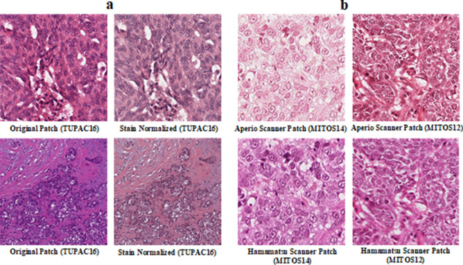
Figure 3
( a ) Actual vs. stain normalized images; ( b ) histopathological images from different scanners.

Figure 4
( a ) Pixel-level annotations; ( b ) weak labels (centroid labels).
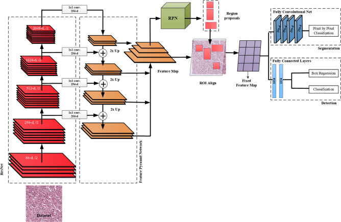
Figure 5
Architectural details of the Mask R-CNN.
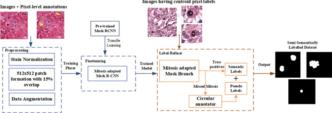
Figure 6
Label refinement module (label-refiner) for the weakly annotated dataset.
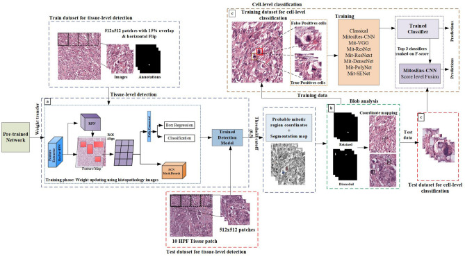
Figure 7
Work flow diagram, ( a ) mitotic region selection at tissue-level using multi-objective deep instance based detection and segmentation model, ( b ) blob analysis, ( c ), enhancement using cell-level c...
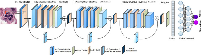
Figure 8
Block diagram of the proposed MitosRes-CNN.
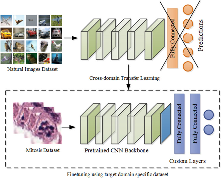
Figure 9
Cross-domain TL of the state-of-the-art CNN architectures.
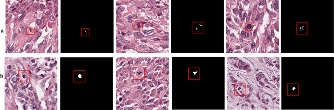
Figure 10
( a ) Annotation results from blue-ratio binary thresholding (threshold valueu2009=u20090.0075), panel ( b ) results of the proposed label-refiner that generates the pixel level image labels.
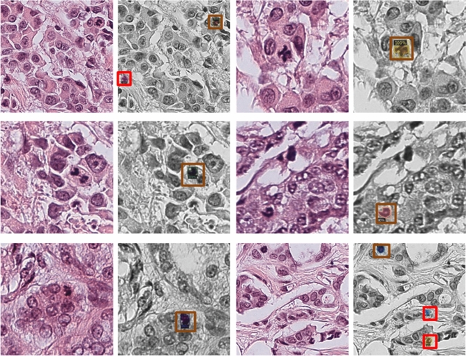
Figure 11
Results of the mitosis detection module at tissue-level, orange box highlights the true predictions whereas red box shows the false positive predictions (non-mitosis).
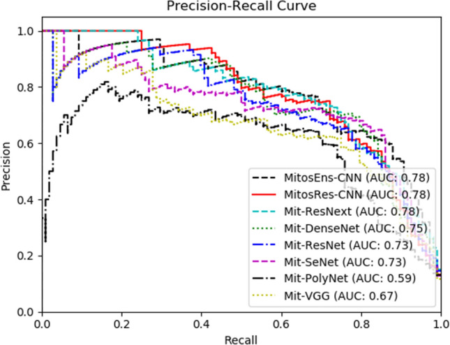
Figure 12
Discrimination analysis via PR curve.
Figure images are served from the NIH/NLM PubMed Central Open Access Subset or Europe PMC; copyright remains with the publishers and authors.
💬 Discussion
0 commentsNo comments yet. Be the first to start a discussion!
Leave a Comment