Abstract
We investigated the neural representation of locomotion in the nematode C. elegans by recording population calcium activity during movement. We report that population activity more accurately decodes locomotion than any single neuron. Relevant signals are distributed across neurons with diverse tunings to locomotion. Two largely distinct subpopulations are informative for decoding velocity and curvature, and different neurons’ activities contribute features relevant for different aspects of a behavior or different instances of a behavioral motif. To validate our measurements, we labeled neurons AVAL and AVAR and found that their activity exhibited expected transients during backward locomotion. Finally, we compared population activity during movement and immobilization. Immobilization alters the correlation structure of neural activity and its dynamics. Some neurons positively correlated with AVA during movement become negatively correlated during immobilization and vice versa. This work provides needed experimental measurements that inform and constrain ongoing efforts to understand population dynamics underlying locomotion in C. elegans .
🔬 Techniques
🧬 Organisms
✨ Fluorophores
🧪 Sample Preparation
💻 Software Details
💻 Code & Software
📂💾 Data Repositories
🏛️ Research Organizations (ROR)
Affiliated research institutions:
📋 Methods
Key resources table
Reagent type (species) or resource Designation Source or reference Identifiers Additional information Strain, strain background ( C. elegans ) AML310 this work Details in Table 2 Strain, strain background ( C. elegans ) AML32 Nguyen et al., 2017 RRID: WBI-STRAIN:WBStrain00000192 Strain, strain background ( C. elegans ) AML18 Nguyen et al., 2016 RRID: WBI-STRAIN:WBStrain00000191 Strains Three strains were used in this study, see Table 2 . AML32 ( Nguyen et al., 2017 ) and AML310 were used for calcium imaging. AML18 ( Nguyen et al., 2016 ) served as a calcium insensitive control. Strain AML310 is similar to AML32 but includes additional labels to identify AVA neurons. AML310 was generated by injecting 30 ng/ul of P rig-3 ::tagBFP plasmid into AML32 strains (wtfIs5[P rab-3 ::NLS ::GCaMP6s; P rab-3 ::NLS::tagRFP]). AML310 worms were selected and maintained by picking individuals expressing BFP fluorescence in the head. Animals were cultivated in the dark on NGM plates with a bacterial lawn of OP50. Table 2. Strains used. Associated Research Resource Identifiers are listed in Key Resources.
Strain Genotype Expression Role Reference
AML310 wtfIs5[P rab-3 ::NLS::GCaMP6s; P rab-3 ::NLS::tagRFP]; wtfEx258 [P rig-3 ::tagBFP::unc-54] tag-RFP and GCaMP6s in neuronal nuclei; BFP in cytoplasm of AVA and some pharyngeal neurons (likely I1, I4, M4 and NSM) Calcium imaging with AVA label This Study AML32 wtfIs5[P rab-3 ::NLS::GCaMP6s; P rab-3 ::NLS::tagRFP] tag-RFP and GCaMP6s in neuronal nuclei Calcium imaging Nguyen et al., 2017 AML18 wtfIs3[P rab-3 ::NLS::GFP, P rab-3 ::NLS::tagRFP] tag-RFP and GFP in neuronal nuclei Control Nguyen et al., 2016 Whole brain imaging Whole brain imaging in moving animals Whole brain imaging of moving animals was performed as described previously ( Nguyen et al., 2016 ). Table 3 lists all recording used in the study, and Table 4 cross-lists the recordings according to figure. Briefly, adult animals were placed on an imaging plate (a modified NGM media lacking cholesterol and with agarose in place of agar) and covered with mineral oil to provide optical index matching to improve contrast for behavior imaging ( Leifer et al., 2011 ). A coverslip was placed on top of the plate with 100 m plastic spacers between the coverglass and plate surface. The coverslip was fixed to the agarose plate with valap. Animals were recorded on a custom whole brain imaging system, which simultaneously records four video streams to image the calcium activity of the brain while simultaneously capturing the animal’s behavior as the animal crawls on agar in two-dimensions. We record ×10 magnification darkfield images of the body posture, ×10x magnification fluorescence images of the head for real-time tracking, and two ×40 magnification image streams of the neurons in the head, one showing tagRFP and one showing either GCaMP6s, GFP, or BFP. The ×10 images are recorded at 50 frames/s, and the 40x fluorescence images are recorded at a rate of 200 optical slices/s, with a resulting acquisition rate of 6 head volumes/s. Recordings were stopped when the animal ran to the edge of the plate, when they left the field of view, or when photobleaching decreased the contrast between tag-RFP and background below a minimum level. Intensity of excitation light for fluorescent imaging was adjusted from recording to recording to achieve different tradeoffs between fluorescence intensity and recording duration. Moving recordings had to meet the following criteria. The animal had to be active and the recording had to be at least 200 s. The tag-RFP neurons also had to be successfully segmented and tracked via our analysis pipeline. Table 3. Recordings used in this study. Unique ID Strain Duration (mins) Notes AML310_A AML310 4 Ca 2+ imaging w/ AVA label, moving AML310_B 4 AML310_C 4 AML310_D 4 AML310_E AML310 8 Ca 2+ imaging w/ AVA label, moving-to-immobile AML310_F 8 AML310_G AML310 15 Ca 2+ imaging w/ AVA label, immobile AML32_A AML32 11 Ca 2+ imaging, moving AML32_B 11 AML32_C 10 AML32_D 11 AML32_E 4 AML32_F 5 AML32_G 4 AML32_H AML32 13 Ca 2+ imaging, moving-to-immobile AML18_A AML18 10 GFP control, moving AML18_B 10 AML18_C 7 AML18_D 5 AML18_E 5 AML18_F 6 AML18_G 9 AML18_H 6 AML18_I 7 AML18_J 6 AML18_K 6 Table 4. List of recordings included in each figure. Figure Recordings Figure 1 ; Figure 1—figure supplement 1 ; Figure 1—figure supplement 2 ; AML310_A Figure 1—figure supplement 3 AML310_A-D, AML32_A-G, AML18_A-K Figure 2a,b ; Figure 2—figure supplement 1 AML310_A Figure 2c AML310_A-D Figure 3a–d AML310_A Figure 3e,f AML310_A-D, AML32_A-G, AML18_A-K Figure 3—figure supplement 1 ; Figure 3—figure supplement 2 ; Figure 3—figure supplement 4 ; Figure 3—figure supplement 5 AML310_A-D, AML32_A-G Figure 3—figure supplement 3 AML18_A-K Figure 4 AML32_A Figure 5 ; Figure 5—figure supplement 1 ; Figure 5—figure supplement 2 AML310_A Figure 5—figure supplement 3 AML32_A Figure 6a,b ; Figure 6—video 1 AML310_A Figure 6c AML310_A-D, AML32_A-G Figure 7a–f AML310_E Figure 7g AML310_A-F, AML32_A-H Figure 7—figure supplement 1 AML32_H Figure 7—figure supplement 2 AML310_G Figure 8 AML310_E Moving to immobile transition experiments Adult animals were placed in a PDMS microfluidic artificial dirt style chip ( Lockery et al., 2008 ) filled with M9 medium where the animal could crawl. The chip was imaged on the whole brain imaging system. A computer controlled microfluidic pump system delivered either M9 buffer or M9 buffer with the paralytic levamisole or tetramisole to the microfluidic chip. Calcium activity was recorded from the worm as M9 buffer flowed through the chip with a flow rate of order a milliliter a minute. Partway through the recording, the drug buffer mixture was delivered at the same flow rate. At the conclusion of the experiment for AML310 worms, BFP was imaged. Different drug concentrations were tried for different recordings to find a good balance between rapidly immobilizing the animal without also inducing the animal to contract and deform. Paralytic concentrations used were: 400 μM for AML310_E, 100 μM for AML310_F, and 5 μM for AML32_H. Recordings were performed until a recording achieved the following criteria for inclusion: (1) the animal showed robust locomotion during the moving portion of the recording, including multiple reversals. (2) The animal quickly immobilized upon application of the drug. (3) The animal remained immobilized for the remainder of the recording except for occasional twitches, (4) the immobilization portion of the recording was of sufficient duration to allow us to see multiple cycles of the stereotyped neural state space trajectories if present and (5) for strain AML310, neurons AVAL and AVAR were required to be visible and tracked throughout the entirety of the recording. For the statistics of correlation structure in Figure 7f , recording AML310_F was also included even though it did not meet all criteria (it lacked obvious reversals).
Show full methods section
Key resources table
Reagent type (species) or resource Designation Source or reference Identifiers Additional information Strain, strain background ( C. elegans ) AML310 this work Details in Table 2 Strain, strain background ( C. elegans ) AML32 Nguyen et al., 2017 RRID: WBI-STRAIN:WBStrain00000192 Strain, strain background ( C. elegans ) AML18 Nguyen et al., 2016 RRID: WBI-STRAIN:WBStrain00000191 Strains Three strains were used in this study, see Table 2 . AML32 ( Nguyen et al., 2017 ) and AML310 were used for calcium imaging. AML18 ( Nguyen et al., 2016 ) served as a calcium insensitive control. Strain AML310 is similar to AML32 but includes additional labels to identify AVA neurons. AML310 was generated by injecting 30 ng/ul of P rig-3 ::tagBFP plasmid into AML32 strains (wtfIs5[P rab-3 ::NLS ::GCaMP6s; P rab-3 ::NLS::tagRFP]). AML310 worms were selected and maintained by picking individuals expressing BFP fluorescence in the head. Animals were cultivated in the dark on NGM plates with a bacterial lawn of OP50. Table 2. Strains used. Associated Research Resource Identifiers are listed in Key Resources.
Strain Genotype Expression Role Reference
AML310 wtfIs5[P rab-3 ::NLS::GCaMP6s; P rab-3 ::NLS::tagRFP]; wtfEx258 [P rig-3 ::tagBFP::unc-54] tag-RFP and GCaMP6s in neuronal nuclei; BFP in cytoplasm of AVA and some pharyngeal neurons (likely I1, I4, M4 and NSM) Calcium imaging with AVA label This Study AML32 wtfIs5[P rab-3 ::NLS::GCaMP6s; P rab-3 ::NLS::tagRFP] tag-RFP and GCaMP6s in neuronal nuclei Calcium imaging Nguyen et al., 2017 AML18 wtfIs3[P rab-3 ::NLS::GFP, P rab-3 ::NLS::tagRFP] tag-RFP and GFP in neuronal nuclei Control Nguyen et al., 2016 Whole brain imaging Whole brain imaging in moving animals Whole brain imaging of moving animals was performed as described previously ( Nguyen et al., 2016 ). Table 3 lists all recording used in the study, and Table 4 cross-lists the recordings according to figure. Briefly, adult animals were placed on an imaging plate (a modified NGM media lacking cholesterol and with agarose in place of agar) and covered with mineral oil to provide optical index matching to improve contrast for behavior imaging ( Leifer et al., 2011 ). A coverslip was placed on top of the plate with 100 m plastic spacers between the coverglass and plate surface. The coverslip was fixed to the agarose plate with valap. Animals were recorded on a custom whole brain imaging system, which simultaneously records four video streams to image the calcium activity of the brain while simultaneously capturing the animal’s behavior as the animal crawls on agar in two-dimensions. We record ×10 magnification darkfield images of the body posture, ×10x magnification fluorescence images of the head for real-time tracking, and two ×40 magnification image streams of the neurons in the head, one showing tagRFP and one showing either GCaMP6s, GFP, or BFP. The ×10 images are recorded at 50 frames/s, and the 40x fluorescence images are recorded at a rate of 200 optical slices/s, with a resulting acquisition rate of 6 head volumes/s. Recordings were stopped when the animal ran to the edge of the plate, when they left the field of view, or when photobleaching decreased the contrast between tag-RFP and background below a minimum level. Intensity of excitation light for fluorescent imaging was adjusted from recording to recording to achieve different tradeoffs between fluorescence intensity and recording duration. Moving recordings had to meet the following criteria. The animal had to be active and the recording had to be at least 200 s. The tag-RFP neurons also had to be successfully segmented and tracked via our analysis pipeline. Table 3. Recordings used in this study. Unique ID Strain Duration (mins) Notes AML310_A AML310 4 Ca 2+ imaging w/ AVA label, moving AML310_B 4 AML310_C 4 AML310_D 4 AML310_E AML310 8 Ca 2+ imaging w/ AVA label, moving-to-immobile AML310_F 8 AML310_G AML310 15 Ca 2+ imaging w/ AVA label, immobile AML32_A AML32 11 Ca 2+ imaging, moving AML32_B 11 AML32_C 10 AML32_D 11 AML32_E 4 AML32_F 5 AML32_G 4 AML32_H AML32 13 Ca 2+ imaging, moving-to-immobile AML18_A AML18 10 GFP control, moving AML18_B 10 AML18_C 7 AML18_D 5 AML18_E 5 AML18_F 6 AML18_G 9 AML18_H 6 AML18_I 7 AML18_J 6 AML18_K 6 Table 4. List of recordings included in each figure. Figure Recordings Figure 1 ; Figure 1—figure supplement 1 ; Figure 1—figure supplement 2 ; AML310_A Figure 1—figure supplement 3 AML310_A-D, AML32_A-G, AML18_A-K Figure 2a,b ; Figure 2—figure supplement 1 AML310_A Figure 2c AML310_A-D Figure 3a–d AML310_A Figure 3e,f AML310_A-D, AML32_A-G, AML18_A-K Figure 3—figure supplement 1 ; Figure 3—figure supplement 2 ; Figure 3—figure supplement 4 ; Figure 3—figure supplement 5 AML310_A-D, AML32_A-G Figure 3—figure supplement 3 AML18_A-K Figure 4 AML32_A Figure 5 ; Figure 5—figure supplement 1 ; Figure 5—figure supplement 2 AML310_A Figure 5—figure supplement 3 AML32_A Figure 6a,b ; Figure 6—video 1 AML310_A Figure 6c AML310_A-D, AML32_A-G Figure 7a–f AML310_E Figure 7g AML310_A-F, AML32_A-H Figure 7—figure supplement 1 AML32_H Figure 7—figure supplement 2 AML310_G Figure 8 AML310_E Moving to immobile transition experiments Adult animals were placed in a PDMS microfluidic artificial dirt style chip ( Lockery et al., 2008 ) filled with M9 medium where the animal could crawl. The chip was imaged on the whole brain imaging system. A computer controlled microfluidic pump system delivered either M9 buffer or M9 buffer with the paralytic levamisole or tetramisole to the microfluidic chip. Calcium activity was recorded from the worm as M9 buffer flowed through the chip with a flow rate of order a milliliter a minute. Partway through the recording, the drug buffer mixture was delivered at the same flow rate. At the conclusion of the experiment for AML310 worms, BFP was imaged. Different drug concentrations were tried for different recordings to find a good balance between rapidly immobilizing the animal without also inducing the animal to contract and deform. Paralytic concentrations used were: 400 μM for AML310_E, 100 μM for AML310_F, and 5 μM for AML32_H. Recordings were performed until a recording achieved the following criteria for inclusion: (1) the animal showed robust locomotion during the moving portion of the recording, including multiple reversals. (2) The animal quickly immobilized upon application of the drug. (3) The animal remained immobilized for the remainder of the recording except for occasional twitches, (4) the immobilization portion of the recording was of sufficient duration to allow us to see multiple cycles of the stereotyped neural state space trajectories if present and (5) for strain AML310, neurons AVAL and AVAR were required to be visible and tracked throughout the entirety of the recording. For the statistics of correlation structure in Figure 7f , recording AML310_F was also included even though it did not meet all criteria (it lacked obvious reversals).
Whole brain imaging in immobile animals
We performed whole brain imaging in adult animals immobilized with 100 nm polystyrene beads ( Kim et al., 2013 ). The worms were then covered with a glass slide, sealed with valap, and imaged using the Whole Brain Imager. Neuron segmentation, tracking, and fluorescence extraction Neurons were segmented and tracked using the Neuron Registration Vector Encoding (NeRVE) and clustering approach described previously ( Nguyen et al., 2017 ) with minor modifications which are highlighted below. As before, video streams were spatially aligned with beads and then synchronized using light flashes. The animals' posture was extracted using an active contour fit to the ×10 magnification darkfield images. But in a departure from the method in Nguyen et al., 2017 , the high magnification fluorescent images are now straightened using a different centerline extracted directly from the fluorescent images. As in Nguyen et al., 2017 , the neural dynamics were then extracted by segmenting the neuronal nuclei in the red channel and straightening the image according to the body posture. Using repeated clustering, neurons are assigned identities over time. The GCaMP signal was extracted using the neural positions found from tracking. The pipeline returns datasets containing RFP and GCaMP6s fluorescence values for each successfully tracked neuron over time, and the centerline coordinates describing the posture of the animal over time. These are subsequently processed to extract neural activity or behavior features. The paralytic used in moving-to-immobile recordings ( Figure 7 ) caused the animal’s head to contract, which would occasionally confuse our tracking algorithm. In those instances the automated NeRVE tracking and clustering was run separately on the moving and immobile portions of the recording (before and after contraction), and then a human manually tracked neurons during the transition period (1–2 min) so as to stitch the moving and immobile tracks together. Photobleaching correction, outlier detection, and pre-processing The raw extracted RFP or GCaMP fluorescent intensity timeseries were preprocessed to correct for photobleaching. Each time-series was fit to a decaying exponential. Those that were well fit by the exponential were normalized by the exponential and then rescaled to preserve the timeseries’ original mean and variance as in Chen et al., 2019 . Timeseries that were poorly fit by an exponential were left as is. If the majority of neurons in a recording were poorly fit by an exponential, this indicated that the animal may have photobleached prior to the recording and the recording was discarded. Outlier detection was performed to remove transient artifacts from the fluorescent time series. Fluorescent time points were flagged as outliers and omitted if they met any of the following conditions: the fluorescence deviated from the mean by a certain number of standard deviations ( F < - 2 σ or F > 5 σ for RFP; | F | > 5 σ for GCaMP); the RFP fluorescence dropped below a threshold; the ratio of GCaMP to RFP fluorescence dropped below a threshold; a fluorescence timepoint was both preceded by and succeeded by missing timepoints or values deemed to be outliers; or if the majority of other neurons measured during the same volume were also deemed to be outliers. Fluorescent time series were smoothed by convolution with a Gaussian ( σ = 0.83 s) after interpolation. Omitted time points, or gaps where the neuron was not tracked, were excluded from single-neuron analyses, such as the calculation of each neuron’s tuning curve. It was not practical to exclude missing time points from the population-level analyses such as linear decoding. In these population-level analyses, interpolated values were used. Time points in which the majority of neurons had missing fluoresecent values were excluded, even in population level analyses. Those instances are shown as white vertical stripes in the fluorescent activity heatmaps, for example, as visible in Figure 1 . Motion-correction We used the GCaMP fluorescence together with the RFP fluorescence to calculate a motion corrected fluorescence, F m c used through the paper. Note sometimes the subscript mc is omitted for brevity. Motion and deformation in the animal’s head introduce artifacts into the fluorescent time-series. We assume that these artifacts are common to both GCaMP and RFP fluorescence, up to a scale factor, because both experience the same motion. For example, if a neuron is compressed during a head bend, the density of both GCaMP and RFP should increase, causing an increase in the fluorescence in both time-series. We expect that the RFP time series is entirely dominated by artifacts because, in the absence of motion, the RFP fluorescent intensity would be constant. If we further assume that motion artifacts are additive, then a simple correction follows naturally. To correct for motion in the GCaMP fluorescence G , we subtract off a scaled RFP fluorescence, R , (2) F mc = ( G - α R ) - ⟨ G - α R ⟩ , where α is a scaling factor that is fit for each neuron so as to minimize ∑ ( G ( t ) - α R ( t ) ) 2 . This approach has similarities to Tai et al., 2004 . The final motion corrected signal F mc is mean-subtracted. When presenting heatmaps of calcium activity, we use the colormap to convey information about the relative presence of calcium activity compared to motion artifact in the underlying recording. The limits on the colormap are determined by the uncorrected green fluorescent timeseries, specifically the 99th percentile of ± | G - ⟨ G ⟩ | of all neurons at all time points in the recording. With this colormap, recordings in which the neurons contain little signal compared to motion artifact will appear dim, while recordings in which neurons contain signal with large dynamics compared to the motion artifact will appear bright. Temporal derivative The temporal derivatives of motion corrected neuron signals are estimated using a Gaussian derivative kernel of width 2.3 s. For brevity we denote this kernel-based estimate as d F d t . Identifying AVA AVAL and AVAR were identified in recordings of AML310 by their known location and the presence of a BFP fluorescent label expressed under the control of the rig-3 promoter. BFP was imaged immediately after calcium imaging was completed, usually while the worm was still moving. To image BFP, a 488 nm laser was blocked and the worm was then illuminated with 405 nm laser light. In one of the recordings, only one of the two AVA neurons was clearly identifiable throughout the duration of the recording. For that recording, only one of the AVA neurons was included in analysis. Measuring and representing locomotion To measure the animal’s velocity v , we first find the velocity vector that describes the motion of a point on the animal’s centerline 15% of its body length back from the tip of its head. We then project this velocity vector onto a head direction vector of unit length. The head direction is taken to be the direction between two points along the animal’s centerline, 10% and 20% posterior of the tip of the head. To calculate this velocity, the centerline and stage position measurements were first Hampel filtered and then interpolated onto a common time axis of 200 Hz (the rate at which we query stage position). Velocity was then obtained by convolving the position with the derivative of a Gaussian with σ = 0.5 s. To measure the animal’s average curvature ⟨ κ ⟩ at each time point, we calculated the curvature d θ / d s at each of 100 segments along the worm’s centerline, where s refers to the arc length of the centerline. We then took the mean of the curvatures of the middle segments that span an anterior-posterior region from 15% to 80% along the animal’s centerline. This region was chosen to exclude curvature from small nose deflections (sometimes referred to as foraging) and to exclude the curvature of the tip of the tail.
Relating neural activity to behavior
Tuning curves The Pearson’s correlation coefficient ρ is reported for each neurons’ tuning, as in Figure 1d,e . To reject the null hypothesis that a neuron is correlated with behavior by chance we took a shuffling approach and applied a Bonferroni correction for multiple hypothesis testing. We shuffled our data in such a way as to preserve the correlation structure in our recording. To calculate the shuffle, each neuron’s activity was time-reversed and circularly shifted relative to behavior by a random time lag and then the Pearson’s correlation coefficient was computed. Shuffling was repeated for each neuron in a recording M times to build up a distribution of M × N values of ρ, where N is the number of neurons in the recording. For AML310_A, we shuffled each neuron in the recording M = 5000 times. For other datasets we shuffled each neuron M = 500 times. To reject the null hypothesis at 0.05% confidence, we apply a Bonferonni correction such that a correlation coefficient greater than ρ (or less than, depending on the sign) must have been observed in the shuffled distribution with a probability less than 0.05 / ( 2 N ) . The factor of 2 N arises from accounting for multiple hypothesis testing for tuning of both F and d F / d t for each neuron.
Population model
We use a ridge regression ( Hoerl and Kennard, 1970 ) model to decode behavior signals y ( t ) (the velocity and the body curvature). The model prediction is given by a linear combination of neural activities and their time derivatives, (3) y ^ ( t ) = ∑ i ( W F , i F i ( t ) + W d F d t , i d F i d t ( t ) ) + β . Note here we are omitting the mc subscript for convenience, but these still refer to the motion corrected fluorescence signal. We scale all these features to have zero mean and unit variance, so that the magnitudes of weights can be compared to each other. To determine the parameters { W F , i , W d F d t , i , β } , we hold out a test set comprising the middle 40% of the recording, and use the remainder of the data for training. We minimize the cost function (4) C = ∑ t ∈ Train ( y ( t ) - y ^ ( t ) ) 2 + λ ∑ i ( W F , i 2 + W d F d t , i 2 ) . The hyperparameter λ sets the strength of the ridge penalty in the second term. We choose λ by splitting the training set further into a second training set and a cross-validation set, and training on the second training set with various values of λ. We choose the value which gives the best performance on the cross-validation set. To evaluate the performance of our model, we use a mean-subtracted coefficient of determination metric, R MS 2 , on the test set. This is defined by (5) R MS 2 ( y , y ^ ) = R 2 ( y - ⟨ y ⟩ , y ^ - ⟨ y ^ ⟩ ) , where we use the conventional definition of R 2 , defined here for an arbitrary true signal z and corresponding model prediction z ^ : (6) R 2 ( z , z ^ ) = 1 - ∑ t ∈ Test ( z ( t ) - z ^ ( t ) ) 2 ∑ t ∈ Test ( z ( t ) - ⟨ z ( t ) ⟩ ) 2 . Note that R MS 2 can take any value on ( - ∞ , 1 ] .
Restricted models
To assess the distribution of locomotive information throughout the animal’s brain, we compare with two types of restricted models. First, we use a Best Single Neuron model in which all but one of the coefficients { W F , i , W d F d t , i } in Equation (3) are constrained to vanish. We thus attempt to represent behavior as a linear function of a single neural activity, or its time derivative These models are shown in Figure 3 . Second, after training the population model, we sort the neurons in descending order of max ( | W F , i | , | W d F d t , i | ) . We then construct models using a subset of the most highly weighted neurons, with the relative weights on their activities and time derivatives fixed by those used in the population model. The performance of these truncated models can be tabulated as a function of the number of neurons included to first achieve a given performance, as shown in Figure 6 . Note that when reporting fraction of total model performance for this partial model, we evaluate performance on the entire dataset (held-out and training, denoted R MS,all 2 ) because all relative weights for the model have already been frozen in place and there is no risk of overfitting.
Alternative models
The population model used throughout this work refers to a linear model with derivatives using ridge regression. In Figure 3—figure supplement 4 , we show the performance of seven alternative population models at decoding velocity for our exemplar recording. The models are summarized in Table 5 . Many of these models perform similarly to the linear population model used throughout the paper. Our chosen model was selected both for its relative simplicity and because it showed one of the highest mean performances at decoding velocity across recordings. Table 5. Alternative models explored. Most are linear models, using either the Ridge or ElasticNet regularization. In some cases, we add an additional term to the cost function which penalizes errors in the temporal derivative of model output (which, for velocity models, corresponds to the error in the predicted acceleration). For features, we use either the neural activities alone, or the neural activities together with their temporal derivatives. We also explore two nonlinear models: MARS Friedman, 1991 , and a shallow decision tree which chooses between two linear models. Model Penalty Features Number of parameters Linear Ridge F and d F / d t 2 N n + 1 Linear Ridge F N n + 1 Linear Ridge + Acceleration Penalty F and d F / d t 2 N n + 1 Linear Ridge + Acceleration Penalty F N n + 1 Linear ElasticNet F and d F / d t 2 N n + 1 Linear ElasticNet F N n + 1 MARS (nonlinear) MARS F and d F / d t variable Linear with Decision Tree (nonlinear) Ridge F and d F / d t 4 N n + 9 Figure 3—figure supplement 4a–b show the model we use throughout the paper, and the same model but with only fluorescence signals (and not their time derivatives) as features. The latter model attains a slightly lower score of R MS 2 = 0.60 . Note that while adding features is guaranteed to improve performance on the training set, performance on the held-out test set did not necessarily have to improve. Nonetheless, we generally found that including the time derivatives led to better predictions on the test set. Figure 3—figure supplement 4c–d show a variant of the linear model where we add an acceleration penalty to the model error. Our cost function becomes ( Equation 4 ). (7) C = ∑ t ∈ Train ( ( y ( t ) - y ^ ( t ) ) 2 + μ ( d y d t ( t ) - d y ^ d t ( t ) ) 2 ) + λ ∑ i ( W F , i 2 + W d F d t , i 2 ) , where the derivatives d y d t and d y ^ d t are estimated using a Gaussian derivative filter. The parameter μ is set to 10. For our exemplar recording, adding the acceleration penalty hurts the model when derivatives are not included as features, but has little effect when they are. Figure 3—figure supplement 4e–f show a variant where we use an ElasticNet penalty instead of a ridge penalty ( Zou and Hastie, 2005 ). If we write the ridge penalty as the L 2 norm of the weight vector, so that (8) λ ∑ i ( W F , i 2 + W d F d t , i 2 ) ≡ λ ∥ W ∥ 2 2 , the ElasticNet penalty is defined by (9) λ ( r ∥ W ∥ 1 + ( 1 - r ) ∥ W ∥ 2 2 ) , where (10) ∥ W ∥ 1 = ∑ i ( | W F , i | + | W d F d t , i | ) is the L 1 norm of the weight vector. The quantity r is known as the L 1 ratio, and in Figure 3—figure supplement 4 it is set to 10 −2 . We have also tried setting r via cross-validation, and found similar results. Figure 3—figure supplement 4g uses the multivariate adaptive regression splines (MARS) model ( Friedman, 1991 ). The MARS model incorporates nonlinearity by using rectified linear functions of the features, or products of such functions. Generally, they have the advantage of being more flexible than linear models while remaining more interpretable than a neural network or other more complicated nonlinear model. However, we find that MARS somewhat underperforms a linear model on our data. Figure 3—figure supplement 4h uses a decision tree classifier trained to separate the data into forward-moving and backward-moving components, and then trains separate linear models on each component. For our exemplar recording, this model performs slightly better than the model we use throughout the paper. This is likely a result of the clear AVAR signal in Figure 2 , which can be used by the classifier to find the backward-moving portions of the data. Across all our recordings, this model underperforms the simple linear model.
Correlation structure analysis
The correlation structure of neural activity was visualised as the correlation matrix, ρ i , j . To observe changes in correlation structure, a correlation matrix for the moving portion of the recording was calculated separately from the immobile portion. The time immediately following delivery of the paralytic when the animal was not yet paralzed was excluded (usually one to two minutes). To quantify the magnitude of the change in correlation structure, a dissimilarity metric was defined as the root mean-squared change in each neuron’s pairwise correlations, ⟨ ( ρ i , j ′ - ρ i , j ) 2 ⟩ . As a control, changes to correlation structure were measured in moving animals. In this case the correlation structure of the first 30% of the recording was compared to the correlation structure of latter 60% of the recording, so as to mimic the relative timing in the moving-to-immobile recordings.
Software
Analysis scripts are available at https://github.com/leiferlab/PredictionCode ( Leifer, 2021 , copy archived at swh:1:rev:ca59416112a9c10a8d6a3179092a7d3c888bcd4e ).
Data
Data from all experiments including calcium activity traces and animal pose and position are publicly available at https://doi.org/10.17605/OSF.IO/DPR3H .
Additional files Transparent reporting form
📊 Figures
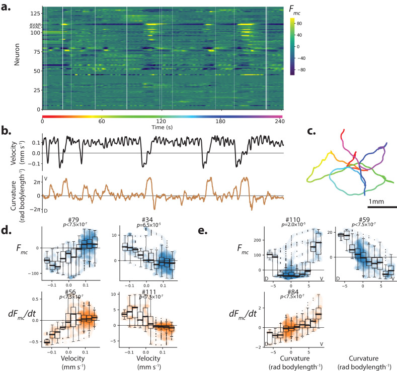
Figure 1.
Population calcium activity and tuning of select neurons during spontaneous animal movement.
Recording AML310_A. ( a ) Calcium activity of 134 neurons is simultaneously recorded during locomotion. Activity is displayed as motion-corrected fluorescent intensity F m u2062 c . Neurons are number...
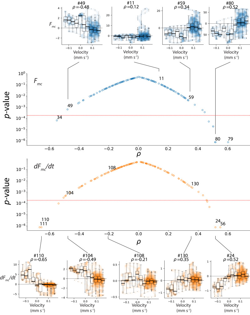
Figure 1u2014figure supplement 1.
Additional details and examples of velocity tuning.
Additional examples of velocity tuning curves for F mc (top) and d u2062 F mc / d u2062 t (bottom) from recording AML310_A are shown. The correlation coefficient u03c1 captures the relation between ea...
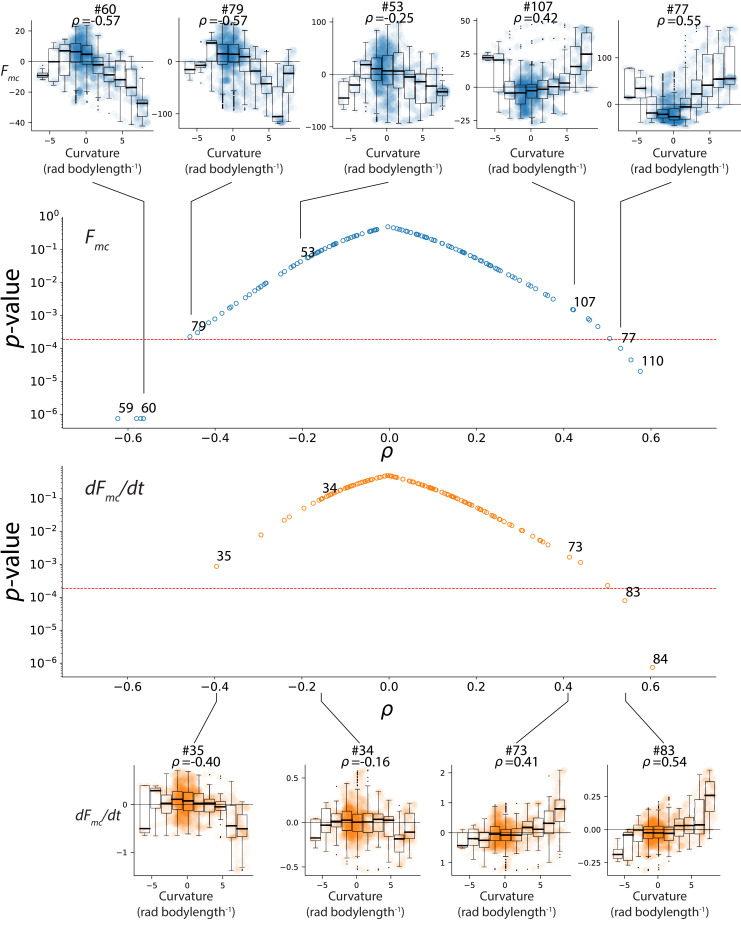
Figure 1u2014figure supplement 2.
Additional details and examples of curvature tuning.
Additional examples of curvature tuning for F mc (top) and d u2062 F mc / d u2062 t (bottom) from recording AML310_A are shown. The correlation coefficient u03c1 captures the relation between each neu...
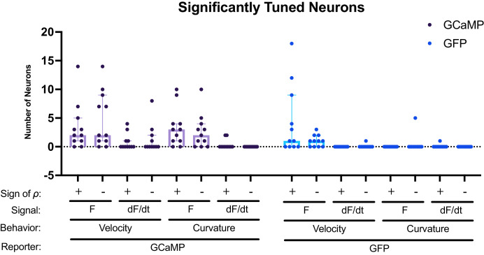
Figure 1u2014figure supplement 3.
Number of significantly tuned neurons across recordings.
Pearsonu2019s correlation coefficient u03c1 was calculated for each neuron in 11 GCaMP recordings and 11 GFP control recordings that lacked a calcium indicator. Neurons were counted as significantly t...
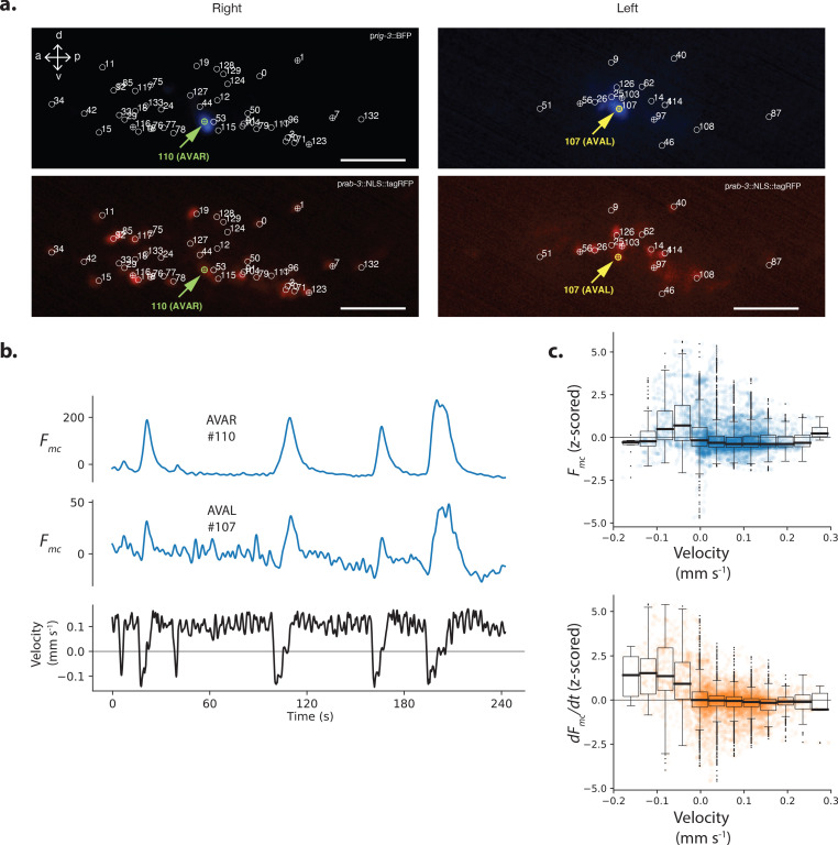
Figure 2.
Neuron pair AVA is active during backward locomotion and exhibits expected tuning during moving population recordings.
( a ) AVAR and AVAL are labeled by BFP under a rig-3 promoter in strain AML310. Two optical planes are shown from a single volume recorded during movement. Planes are near the top and bottom of the op...
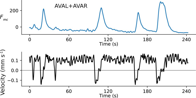
Figure 2u2014figure supplement 1.
Sum of AVAL and AVAR activity.
Activity of AVAL and AVAR from AML310_A in Figure 2b are shown summed together. This permits comparison to recordings that do not resolve the two neurons separately.
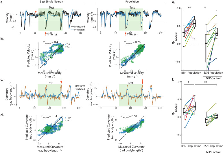
Figure 3.
Population neural activity decodes locomotion.
( au2013d ) Performance of the best single neuron (BSN) is compared to a linear population model in decoding velocity and body curvature for the exemplar recording AML310_A shown in Figure 1 . ( a ) P...
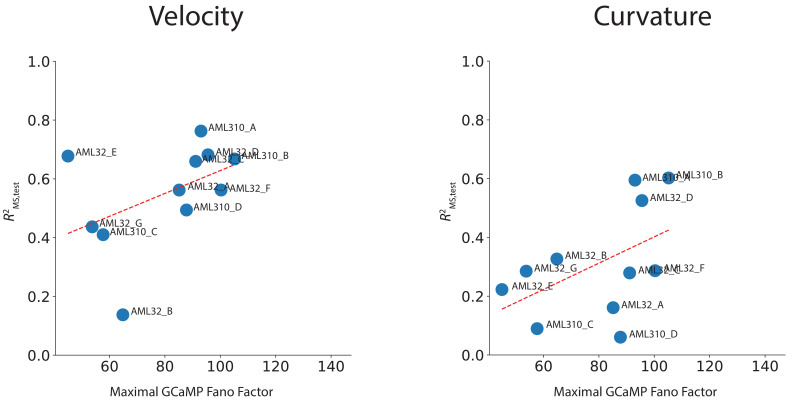
Figure 3u2014figure supplement 1.
Performance correlates with maximal GCaMP Fano Factor, a metric of signal.
Decoding performance is plotted against maximal GCaMP Fano Factor for each recording for velocity and curvature. Maximal GCaMP Fano Factor is the Fano Factor of the raw GCaMP activity for the neuron i...
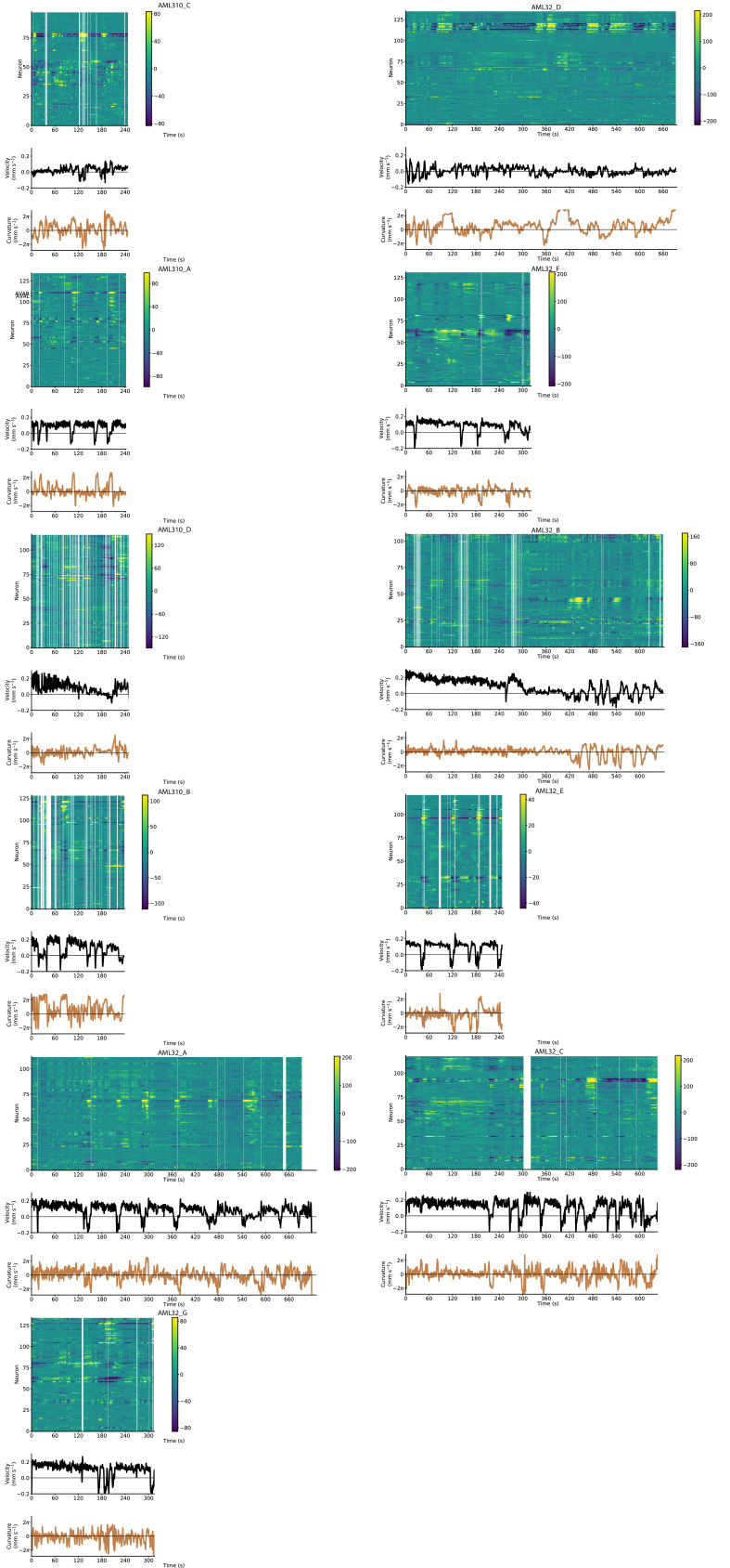
Figure 3u2014figure supplement 2.
Neural activity and behavior for all moving calcium imaging recordings (AML310 and AML32).
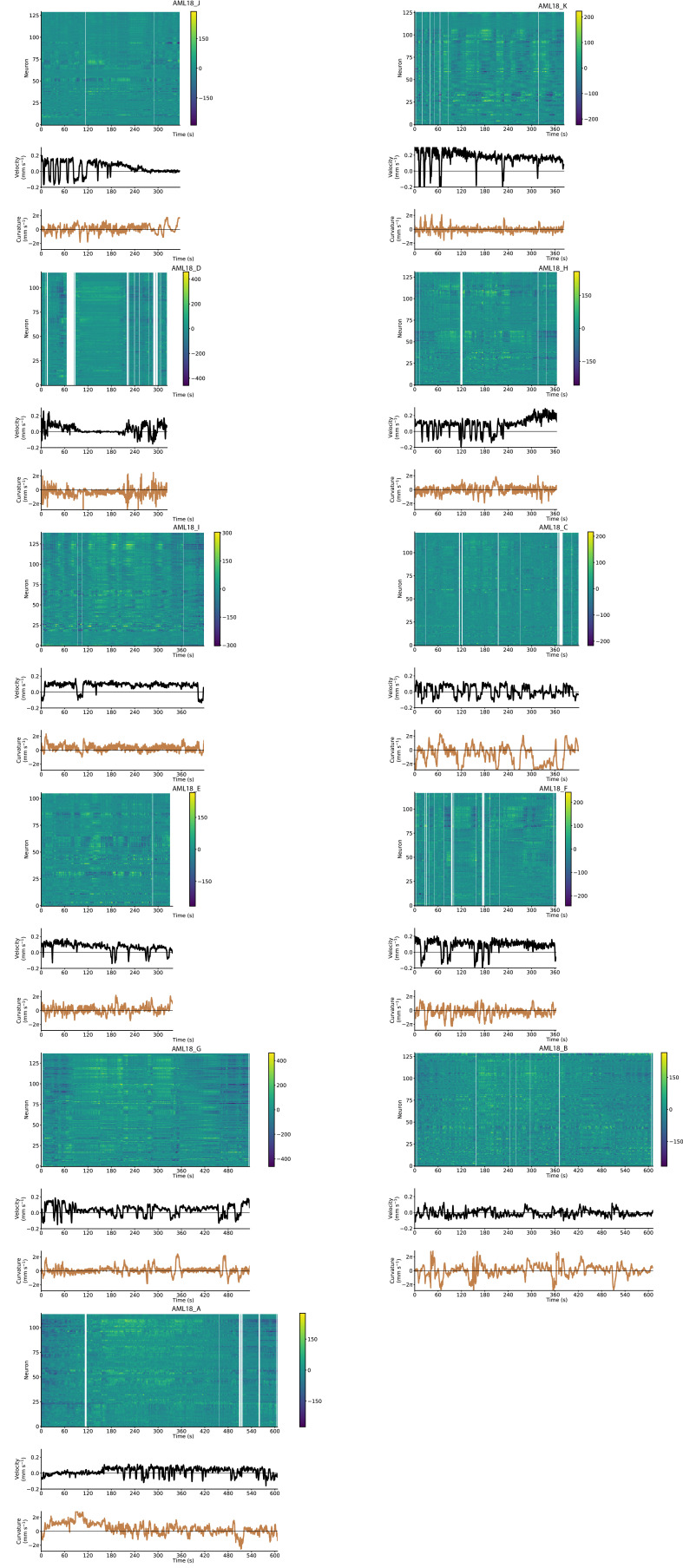
Figure 3u2014figure supplement 3.
Neural activity and behavior for all moving GFP control recordings (AML18).
Neural activity and behavior for all moving GFP control recordings (AML18).
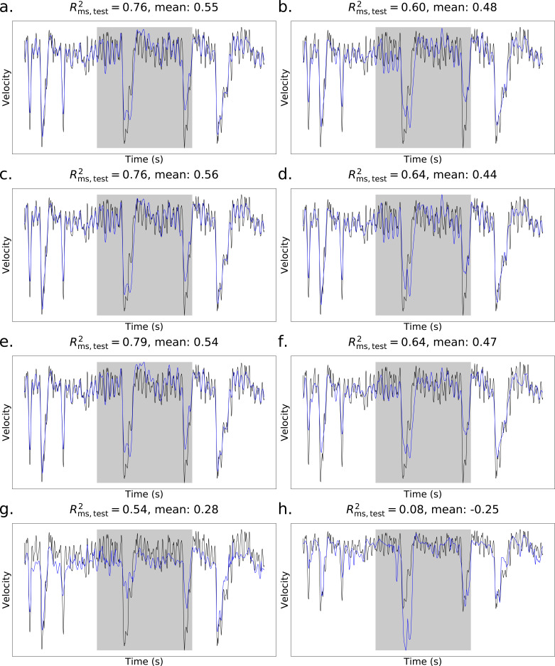
Figure 3u2014figure supplement 4.
Alternative population models.
Performance of alternative population models for decoding velocity. Traces are shown for exemplar recording AML310_A. Mean across all moving GCaMP recordings is also listed. Gray shading shows held-ou...
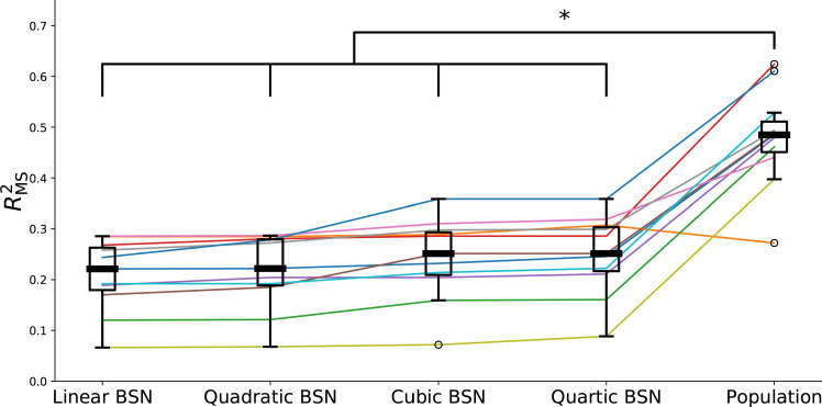
Figure 3u2014figure supplement 5.
Nonlinear fits using best single neuron.
Performance of polynomial regression models for decoding velocity on 11 GCaMP recordings using the best single neuron. The best single neuron is defined as the one with the best decoding performance u...
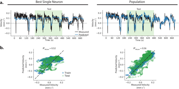
Figure 4.
Example where population decoded a fuller range of animal behavior.
( a ) The decoding from the best single neuron and the population model are compared to the measured velocity for example recordingu00a0AML32_A. ( b ) Predictions from the best single neuron saturate ...
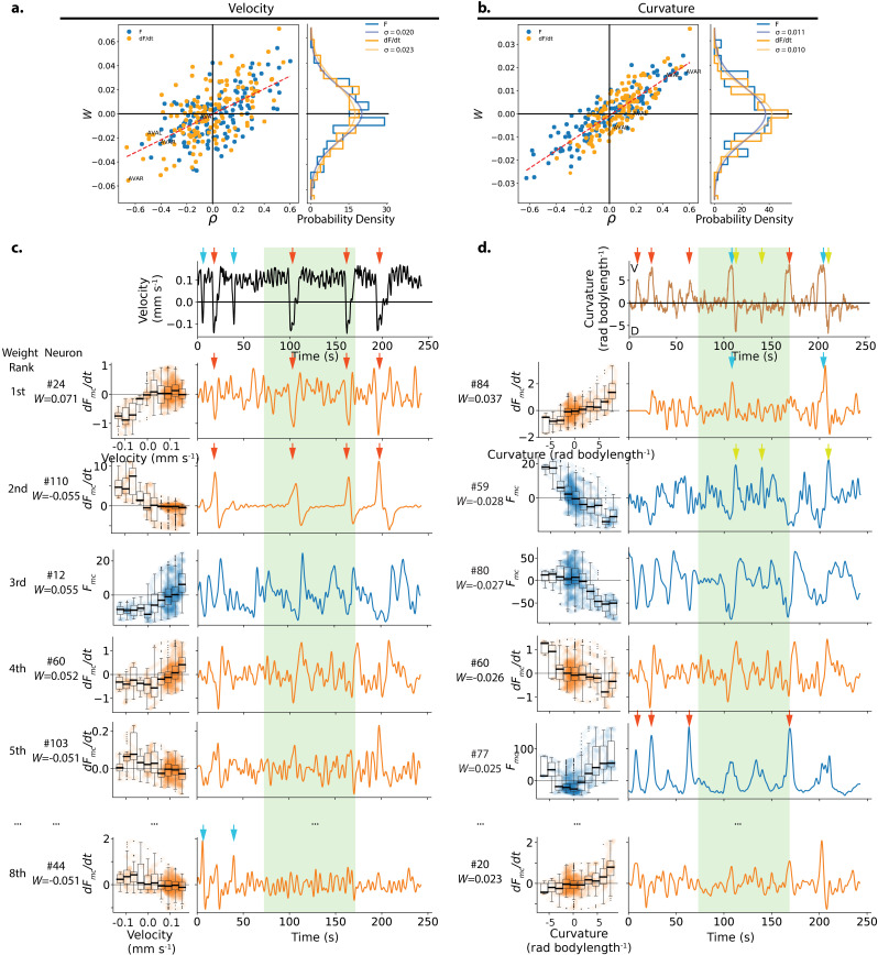
Figure 5.
Weights assigned to neurons by the population model in the exemplar recording, and their respective tuning.
( a ) The weight W assigned to each neuronu2019s activity ( F mc ) or its temporal derivative ( d u2062 F mc / d u2062 t ) by the velocity population decoder is plotted against its Pearsonu2019s Corre...
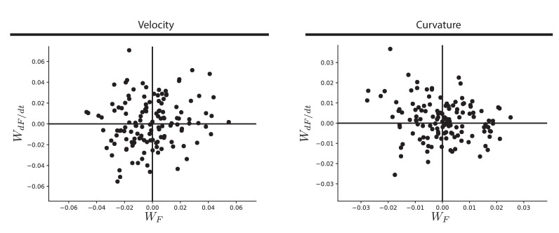
Figure 5u2014figure supplement 1.
Comparison of weights assigned to a neuronu2019s activity versus its temporal derivative.
Comparison of weights assigned to a neuronu2019s activity versus its temporal derivative for velocity (left) or curvature (right) decoders. Comparison of weights assigned to a neuronu2019s activity | ...
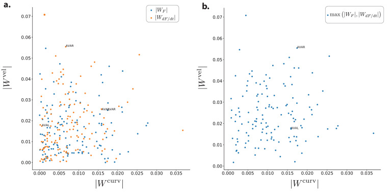
Figure 5u2014figure supplement 2.
Comparison of weights assigned for decoding velocity vs decoding curvature.
Comparison of weights assigned for decoding velocity vs decoding curvature. ( a ) The magnitude of the weight assigned to each neuron in recording AML310_A for velocity | W vel | is compared to the ma...
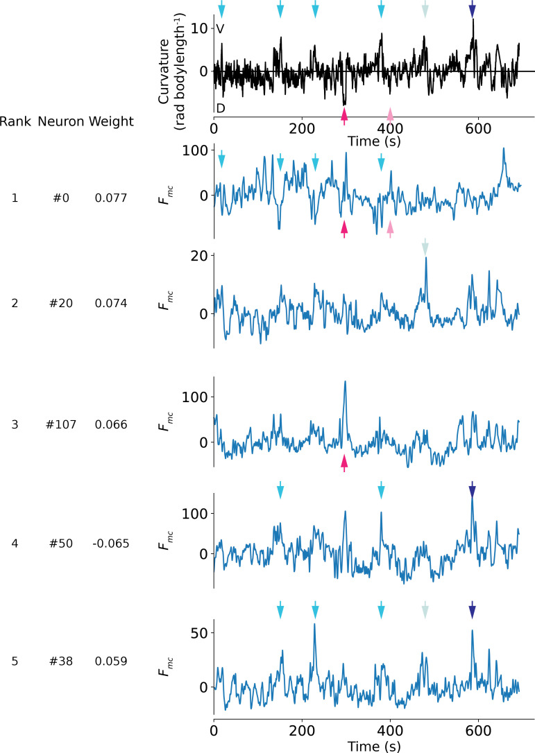
Figure 5u2014figure supplement 3.
Example traces of highly weighted neurons used to decode curvature in AML32_A.
Traces of top five highest weighted neurons used to decode curvature in AML32_A. Same recording as in Figure 4 . Arrows indicate activity peaks corresponding to ventral (blue shades, top) or dorsal tu...
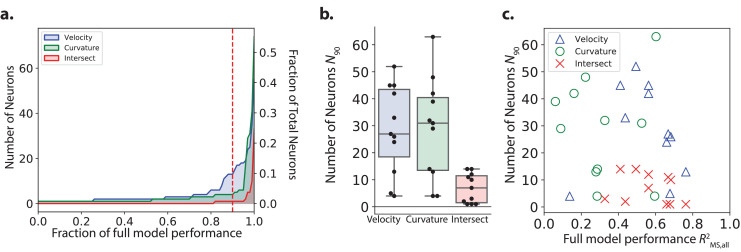
Figure 6.
Number of neurons needed by the model to decode velocity and curvature.
( a ) The minimum number of neurons needed for a restricted model to first achieve a given performance is plotted from recording AML310_A in Figure 1 . Performance, R MS,all 2 is reported separately f...
Figure 6u2014video 1.
Animation showing partial model performance as neurons are added, corresponding to Figure 6a .
Top panel shows performance R MS,all 2 evaluated on both test and training set. Bottom left shows measured velocity (black) and decoded velocity (blue). Gray shading indicates test set. Bottom right s...
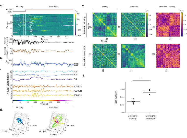
Figure 7.
Immobilization alters the correlation structure of neural activity.
( a ) Calcium activity is recorded from an animal as it moves and then is immobilized with a paralytic drug, recording AML310_E. ( b ) Activity of AVAL and AVAR from ( a ). ( c ) Population activity (...
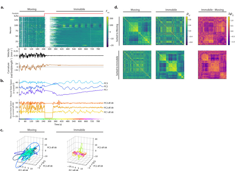
Figure 7u2014figure supplement 1.
Example from additional moving-to-immobile recording.
Calcium activity is recorded from an animal as it moves and then is immobilized with a paralytic drug, recording AML32_H. Activity and behavior. ( b ) Population activity (or its derivative) from ( a ...
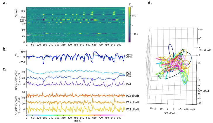
Figure 7u2014figure supplement 2.
Immobile-only recording.
Calcium activity is recorded from an animal immobilized with nano-beads, recording AML310_G. ( a ) Calcium activity. ( b ) Activity of neurons AVAL and AVAR. ( c ) Population activity (or its temporal...
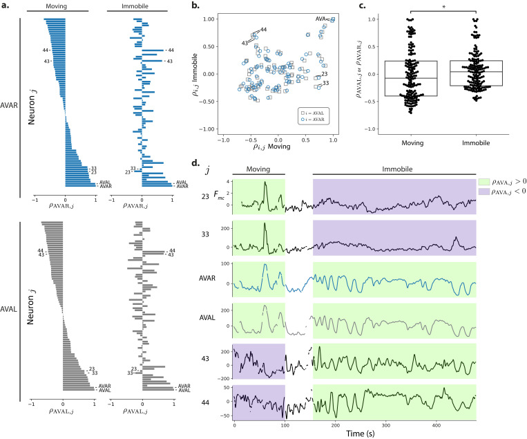
Figure 8.
Correlations with respect to AVAL and AVAR during movement and immobilization.
( a ) The Pearsonu2019s correlation of each neuronu2019s activity to AVAR and AVAL is shown during movement and immobilization. Selected neurons are numbered as in Figure 7 (same recording, AML310_E)....
Figure images are served from the NIH/NLM PubMed Central Open Access Subset or Europe PMC; copyright remains with the publishers and authors.
💬 Discussion
0 commentsNo comments yet. Be the first to start a discussion!
Leave a Comment