Abstract
AbstractGiven the difficulties inherent in maintaining human pluripotent stem cells (hPSCs) in a healthy state, hPSCs should be routinely characterized using several established standard criteria during expansion for research or therapeutic purposes. hPSC colony morphology is typically considered an important criterion, but it is not evaluated quantitatively. Thus, we designed an unbiased method to evaluate hPSC colony morphology. This method involves a combination of automated non-labelled live-cell imaging and the implementation of morphological colony analysis algorithms with multiple parameters. To validate the utility of the quantitative evaluation method, a parent cell line exhibiting typical embryonic stem cell (ESC)-like morphology and an aberrant hPSC subclone demonstrating unusual colony morphology were used as models. According to statistical colony classification based on morphological parameters, colonies containing readily discernible areas of differentiation constituted a major classification cluster and were distinguishable from typical ESC-like colonies; similar results were obtained via classification based on global gene expression profiles. Thus, the morphological features of hPSC colonies are closely associated with cellular characteristics. Our quantitative evaluation method provides a biological definition of ‘hPSC colony morphology’, permits the non-invasive monitoring of hPSC conditions and is particularly useful for detecting variations in hPSC heterogeneity.
🔬 Techniques
💻 Software
🧪 Sample Preparation
🔬 Cell Lines
🏭 Microscope Brands
🧪 Reagent Suppliers
💻 Software Details
🏛️ Research Organizations (ROR)
Affiliated research institutions:
📋 Methods
Cells and cell culture
Two hiPSC lines, 201B7 2 and 253G1 3 , and their subclones (201B7-1A and 253G1-B1, respectively) were provided by Dr. Shinya Yamanaka of the Center for iPS Cell Research, Kyoto University. The hiPSC line Tic (JCRB1331) was obtained from the JCRB Cell Bank (NIBIOHN, Ibaraki, Osaka, Japan) 26 27 28 , and the hESC line H9 (WA09) 1 was obtained from the WISC Bank (WiCell Research Institute, Madison, WI, USA). Experiments using hESCs were performed following the guidelines for the utilization of hESCs established by the Ministry of Education, Culture, Sports, Science and Technology, Japan, with the approval of each institutional research ethics committee. Detailed information on the cell lines used in the present study is provided in Supplementary Tables S1–3 . For 201B7 and 201B7-1A, detailed biological characterization is also provided in Supplementary Fig. S1 . For teratoma formation assay in Fig. S1C , iPSCs suspended in DMEM supplemented with ROCK inhibitor were injected into the rear leg muscle or thigh muscle of SCID (C.B-17/lcr-scid/scidJcl) mice (CLEA Japan, Tokyo, Japan) (detail described in the Supplementary Methods ). All animal experiments were conducted in accordance with the institutional and Japanese guidelines for animal experiments, genetic recombination experiments, human iPSC experiments, and hESC experiments after approval by the committee meetings for the animal experiments and the safety for genetic recombination experiments, and the institutional ethical review board of National Institutes of Biomedical Innovation, Health and Nutrition, Osaka, Japan. Cell lines were routinely maintained as reported previously 25 36 44 45 . The details are described in the Supplementary Methods . Tic cells maintained under conventional culture conditions were transferred to feeder-free culture conditions as described in the Supplementary Methods .
Show full methods section
Cells and cell culture
Two hiPSC lines, 201B7 2 and 253G1 3 , and their subclones (201B7-1A and 253G1-B1, respectively) were provided by Dr. Shinya Yamanaka of the Center for iPS Cell Research, Kyoto University. The hiPSC line Tic (JCRB1331) was obtained from the JCRB Cell Bank (NIBIOHN, Ibaraki, Osaka, Japan) 26 27 28 , and the hESC line H9 (WA09) 1 was obtained from the WISC Bank (WiCell Research Institute, Madison, WI, USA). Experiments using hESCs were performed following the guidelines for the utilization of hESCs established by the Ministry of Education, Culture, Sports, Science and Technology, Japan, with the approval of each institutional research ethics committee. Detailed information on the cell lines used in the present study is provided in Supplementary Tables S1–3 . For 201B7 and 201B7-1A, detailed biological characterization is also provided in Supplementary Fig. S1 . For teratoma formation assay in Fig. S1C , iPSCs suspended in DMEM supplemented with ROCK inhibitor were injected into the rear leg muscle or thigh muscle of SCID (C.B-17/lcr-scid/scidJcl) mice (CLEA Japan, Tokyo, Japan) (detail described in the Supplementary Methods ). All animal experiments were conducted in accordance with the institutional and Japanese guidelines for animal experiments, genetic recombination experiments, human iPSC experiments, and hESC experiments after approval by the committee meetings for the animal experiments and the safety for genetic recombination experiments, and the institutional ethical review board of National Institutes of Biomedical Innovation, Health and Nutrition, Osaka, Japan. Cell lines were routinely maintained as reported previously 25 36 44 45 . The details are described in the Supplementary Methods . Tic cells maintained under conventional culture conditions were transferred to feeder-free culture conditions as described in the Supplementary Methods .
Immunohistochemical staining
Immunocytochemistry was performed as described previously 36 . Image analysis was performed using CL-Quant (version 3.0 beta, Nikon, Tokyo, Japan). Primary and secondary antibodies used in the present study are listed in Supplementary Table S13 .
Image acquisition
Phase-contrast colony image acquisition was achieved using a BioStation CT culture incubator, microscope and digital imaging system (Nikon) that was adjusted to optimise the auto-focus and cell image-tiling acquisition functions according to the instructions provided ( Supplementary Fig. S3 ). Colony images were obtained from tissue culture-treated 6-well plates (353046, Becton Dickinson, Franklin Lakes, NJ, USA) at 4 × magnification. The centre of each well was optimized to tile 64 ( = 8 × 8) single-shot images (1,000 × 1,000 pixels 2 , 2,000 × 2,000 μm 2 /image) as the field of view for each well. The optimized field of view covered the maximum area in the 6-well plate to obtain phase-contrast colony images without incorporating any effects of the liquid surface meniscus. Images were saved as PNG files. For the acquisition of all images, the interval was set at 8 h, starting 48 h after seeding to avoid the disruption of colony adhesion. To acquire images to construct the colony database, 4 hiPSC clones (201B7, 201B7-1A, 253G1 and 253G1-B1 at 6 plates/cell clone) were prepared and cultured in the BioStation CT for 6 days (total images obtained = 2,304 images, comprising 64 images from 6–12 wells per clone). To acquire images of the colonies selected for single-colony microarray analyses, 6 plates/clone were freshly prepared approximately 6 months after colony database construction with 201B7 and 201B7-1A and cultured in the BioStation CT for 4 days (total images obtained = 1,536 images, 256 images/plate). All raw images (Ph channel) obtained from the BioStation CT and analytical data are available at https://mega.nz/#!3sJXAYLR!67ksyOiGAz2EjI2QSclNfB3z88u2D-SOvendMbuTTXY (For any additional information about the files, please contact the corresponding author).
Image collection for morphological analysis
The image collection process for morphological analysis is represented in Step 1-1 in Supplementary Fig. S2 . Basic colony image measurements were performed using the image analysis software CL-Quant (version 3.0 beta, Nikon). Colony recognition image processing was carried out as described in the manufacturer’s protocol for CL-Quant (Nikon) (a schematic flow is described in Supplementary Figs S13 and S14 ), utilizing the following steps: (step 1) flattening background (parameter setting: kernel size = 7 pixels and grey value = 90); (step 2) colony recognition via colony texture training with the machine learning algorithm of CL-Quant (choosing the maximum recognition accuracy among 50 training patterns); (step 3) noise reduction (parameter setting: 2,046 pixels, optimized for manual colony counting of 30 images); (step 4) object filling (parameter setting: 30 pixels); (step 5) manual object cleansing (eliminating the labels of colony-like objects that are not actually colonies or are partial images of colonies by confirming them in a phase-contrast image view); and (step 6) size limitation for ‘colony’ selection among objects (>30,000 pixels = 400 μm 2 diameter). Using measured image-processing parameter settings, 999 colonies were recognised (>30,000 pixels/colony, excluding extremely small and immature colonies), specifically 490 colonies for 201B7, 254 colonies for 201B7-1A, 136 colonies for 253G1 and 119 colonies for 253G1-B1. We then narrowed our colony database to colonies >1.0 mm in diameter because colonies 0.98) and parameters with a high coefficient of variation (CV; >30) were eliminated to reduce the risk of multicolinearity. Highly correlated parameters were represented by a single parameter that describes and interprets cellular morphology. Eight major parameters comprising a total of 27 sub-parameters were selected as essential for further analysis ( Supplementary Table S4 ). Parameter 3 is sensitive for detecting the smoothness of a colony outline, and parameter 6 is sensitive for detecting the fibrous points of a colony outline.
Clustering for morphological analysis
The clustering process for morphological analysis is represented in Step 1–3 in Supplementary Fig. S2 . Image data were further analysed for colony database construction. Using the selected colony morphological data (303 colonies described by 8 major parameters), average linkage hierarchical clustering (uncentred correlation) was carried out using the open source clustering software Cluster 3.0 (University Tokyo, Human Genome Center, Tokyo, Japan). The clustering results were exported to a.csv file and then analysed with an original program written in R for further pruning and member analysis. To prune the hierarchical clustering tree into ‘clusters,’ a ‘test of no correlation’ based on Pearson’s correlation coefficient was used. We ensured that ‘similar colonies’ passed the ‘test of no correlation’ and pruned the clustering tree with a correlation coefficient r >0.380863, which is the correlation coefficient ‘r-value’ of the 27 parameters. This r-value corresponded to the t-value (t = 2.059539) with a significance level of >0.05. Such pruning resulted in ‘clusters’ of colonies. Among the clusters, we designated clusters that consisted of >5% of all colonies (>15 colonies) as ‘major clusters’ and the others as ‘minor clusters.’ After clustering, the colony existence ratio was compared between 201B7 and 201B7-1A to identify cluster characteristics that defined a ‘201B7-1A clone’, which typically has a ‘disordered morphology.’ The clusters were then ordered according to the characteristics related to 201B7, major-ness and average colony size ( Supplementary Table S5 ). Only cluster-A demonstrated a characteristic colony existence ratio in which the clustered colony ratio was higher for 201B7-1A than for 201B7.
Image data analysis for colony selection for single-colony microarray
The image data analysis process for colony selection for single-colony microarray is represented in Step 2 in Supplementary Fig. S2 . After seeding hPSCs for 72 h, 1,536 images (covering 48, 56, 64 and 72 h) acquired from a fresh batch of hiPSC cultures were processed and measured using the above image processing and image analysis scheme. Newly analysed colonies from the 72-h images were then categorised into clusters-A through -T by searching for the colonies in the colony database possessing the highest Pearson’s correlation coefficients using an original program written in C. New live colonies were labelled by returning the corresponding ‘cluster’ from the search results in the colony database. Among these newly labelled live colonies with cluster names, single colonies that were separated from other neighbouring colonies and could be easily picked were manually selected as candidate colonies for microarray analysis. RNA was individually extracted from each colony that was mechanically harvested from the culture vessel.
Single-colony microarray analysis
The single-colony microarray analysis process is illustrated in Supplementary Fig. S9 . The 32 selected colonies from cluster-A, cluster-B and cluster-D (to evaluate major clusters) and cluster-I and cluster-J (to evaluate minor clusters) were labelled with colony ID numbers (listed in Supplementary Table S9 ). These colonies were marked under the microscope, and neighbouring colonies were eliminated with a cell scraper. Colonies were lysed with Trizol (Life Technologies, Carlsbad, CA, USA) in a colony ring (7-mm diameter), and total RNA was extracted according to the manufacturer’s protocol. Then, small-scale total RNA was amplified using the WT-Ovation Pico RNA Amplification System (3300-12, Nugen Technologies, Inc., CA, USA) and analysed with a BioAnalyzer (Agilent Technologies, Inc., Santa Clara, CA, USA). SurePrint G3 Human GE microarray kits 8 × 60K ver. 2.0 (G4851A, Agilent Technologies, Inc., San Carlos, CA, USA) were used for microarray analysis carried out by DNA Chip Research, Inc., Yokohama, Japan. Microarray data were analysed with GeneSpringGX (Version 12.1) using the standard operating manual provided by the manufacturer. A 75th percentile shift was selected as the sample normalization scheme, and the standard baseline shift was selected for data normalization. Of the 60,000 probes included in the microarray, 29,445 probes had data suitable for analysis. To statistically analyse selected cluster-related genes, a Benjamini–Hochberg t -test with a
📊 Figures
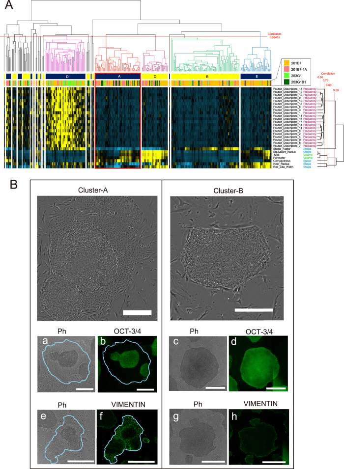
Figure 1
Overview of the morphological varieties and classified colonies of 4 hiPSC clones.
( A ) Clustering of colony morphologies in the colony database according to morphological parameters. Horizontal branches show the hierarchical clustering results divided into 20 clusters at a thresho...
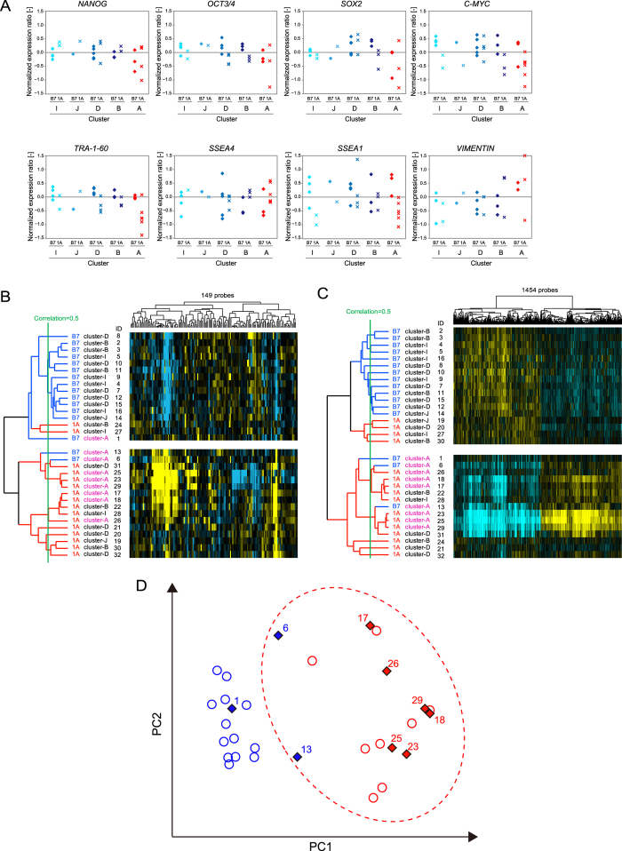
Figure 2
Gene expression profiles of single hiPSC colonies classified as cluster-A, cluster-B, cluster-D, cluster-I and cluster-J 201B7 and 201B7-1A hPSC colonies (32 colonies), classified as cluster-A, cluster-B, cluster-D, cluster-I and cluster-J, were individually picked up from the culture vessel.
RNA extracted from these colonies was used to perform global gene microarray analysis. Gene expression profiles are normalised values, as described in the Methods section. ( A ) Comparisons between 20...
Figure images are served from the NIH/NLM PubMed Central Open Access Subset or Europe PMC; copyright remains with the publishers and authors.
💬 Discussion
0 commentsNo comments yet. Be the first to start a discussion!
Leave a Comment