Abstract
In invertebrate predators such as the praying mantis and vertebrate predators such as wild cats the ability to detect small differences in inter-ocular retinal disparities is a critical means for accurately determining the depth of moving objects such as prey. In mammals, the first neurons along the visual pathway that encode binocular disparities are found in the visual cortex. However, a precise functional architecture for binocular disparity has never been demonstrated in any species, and coarse maps for disparity have been found in only one primate species. Moreover, the dominant approach for assaying the developmental plasticity of binocular cortical neurons used monocular tests of ocular dominance to infer binocular function. The few studies that examined the relationship between ocular dominance and binocular disparity of individual cells used single-unit recordings and have provided conflicting results regarding whether ocular dominance can predict the selectivity or sensitivity to binocular disparity. We used two-photon calcium imaging to sample the response to monocular and binocular visual stimuli from nearly every adjacent neuron in a small region of the cat visual cortex, area 18. Here we show that local circuits for ocular dominance always have smooth and graded transitions from one apparently monocular functional domain to an adjacent binocular region. Most unexpectedly, we discovered a new map in the cat visual cortex that had a precise functional micro-architecture for binocular disparity selectivity. At the level of single cells, ocular dominance was unrelated to binocular disparity selectivity or sensitivity. When the local maps for ocular dominance and binocular disparity both had measurable gradients at a given cortical site, the two gradient directions were orthogonal to each other. Together, these results indicate that, from the perspective of the spiking activity of individual neurons, ocular dominance cannot predict binocular disparity tuning. However, the precise local arrangement of ocular dominance and binocular disparity maps provide new clues regarding how monocular and binocular depth cues may be combined and decoded.
🔬 Techniques
💻 Software
✨ Fluorophores
🧪 Sample Preparation
🏭 Microscope Brands
🔴 Lasers
💻 Software Details
💾 Data Repositories
🏛️ Research Organizations (ROR)
Affiliated research institutions:
📋 Methods
SUMMARY Cats (postnatal days 36–49) were anesthetized with isoflurane (1–2% in surgery, 0.5–1.0% during imaging) 22 and paralyzed with vecuronium bromide 22 . A craniotomy was performed over area 18 of the visual cortex, the dura reflected, and the underlying cortex covered with agarose. Movement of the brain from respiratory and heart beat pulsations were negligible ( Supplementary Fig. S8 ). The cell-permeant calcium indicator Oregon Green 488 Bapta-1 AM (1 mM) was prepared 22 , 30 and co-loaded with 40 μM Alexa Fluor 594 into a glass patch pipette (2.5 μm diameter tip). Under continuous visual guidance, the pipette tip was advanced 200–250 μm below the cortical surface and the indicators were then pressure ejected (5–10 psi). This particular method of loading produces minimal staining of glial cells (see Ref 22 ) but it is possible that some of the stained cells in the present study were not neuronal. Fluorescence was monitored with a custom-built microscope (Prairie Technologies) coupled with a Mai Tai XF (Newport Spectra-Physics) mode-locked Ti:sapphire laser (850 or 920 nm). Drifting sine-wave gratings (2 Hz, 50% contrast) were presented on a CRT (100 Hz refresh rate) in a variety of configurations for orientation, direction of motion, spatial frequency, ocularity (left or right eye—for ocular dominance), and eight inter-ocular spatial phase disparities (0°, 45°, 90°, 135°, 180°, 225°, 270°, 315°). For ocular dominance and binocular disparity assays, animals viewed the monoptic and dichoptic visual stimuli through ultra-fast ferroelectric liquid crystal shutters (7 KHz switching time, 1,000:1 extinction contrast ratio, DisplayTech). Each stimulus period (8 s) was preceded by an equal blank period, repeated 3–8 times. Coarse retinotopic positions of monocular receptive fields were determined by using 5° wide flashing bars of light or strips of gratings at ten retinotopic positions. Two-photon images were analyzed inMatlab (Mathworks)—see Full Methods. Full Methods and any associated references are available in the online version of the paper at www.nature.com/nature .
Show full methods section
SUMMARY Cats (postnatal days 36–49) were anesthetized with isoflurane (1–2% in surgery, 0.5–1.0% during imaging) 22 and paralyzed with vecuronium bromide 22 . A craniotomy was performed over area 18 of the visual cortex, the dura reflected, and the underlying cortex covered with agarose. Movement of the brain from respiratory and heart beat pulsations were negligible ( Supplementary Fig. S8 ). The cell-permeant calcium indicator Oregon Green 488 Bapta-1 AM (1 mM) was prepared 22 , 30 and co-loaded with 40 μM Alexa Fluor 594 into a glass patch pipette (2.5 μm diameter tip). Under continuous visual guidance, the pipette tip was advanced 200–250 μm below the cortical surface and the indicators were then pressure ejected (5–10 psi). This particular method of loading produces minimal staining of glial cells (see Ref 22 ) but it is possible that some of the stained cells in the present study were not neuronal. Fluorescence was monitored with a custom-built microscope (Prairie Technologies) coupled with a Mai Tai XF (Newport Spectra-Physics) mode-locked Ti:sapphire laser (850 or 920 nm). Drifting sine-wave gratings (2 Hz, 50% contrast) were presented on a CRT (100 Hz refresh rate) in a variety of configurations for orientation, direction of motion, spatial frequency, ocularity (left or right eye—for ocular dominance), and eight inter-ocular spatial phase disparities (0°, 45°, 90°, 135°, 180°, 225°, 270°, 315°). For ocular dominance and binocular disparity assays, animals viewed the monoptic and dichoptic visual stimuli through ultra-fast ferroelectric liquid crystal shutters (7 KHz switching time, 1,000:1 extinction contrast ratio, DisplayTech). Each stimulus period (8 s) was preceded by an equal blank period, repeated 3–8 times. Coarse retinotopic positions of monocular receptive fields were determined by using 5° wide flashing bars of light or strips of gratings at ten retinotopic positions. Two-photon images were analyzed inMatlab (Mathworks)—see Full Methods. Full Methods and any associated references are available in the online version of the paper at www.nature.com/nature .
METHODS
Images were analyzed using customized Matlab (Mathworks) software. Cells were identified through a series of morphological filters that defined the contours of cell bodies based on intensity, size, and shape 22 . Time courses of individual cells were extracted by calculating mean pixel values within cell contours 22 . Visually responsive cells were defined by ANOVA across blank and N test visual stimuli ( P < 0.05). Cells selective for particular stimuli were defined by ANOVA across N stimulus periods ( P < 0.05). Ocular dominance (OD) was derived from the responses to monocular stimulation and defined as: O D = R ipsi ( R ipsi + R contra ) Sensitivity to binocular disparity (F1/F0) was derived by vector averaging as follows: V → avg = ∑ i = 1 n V → i n Where V → i is a vector with direction equal to disparity phase, length equal to the corresponding cell’s response amplitude and n is the total number of disparity phases. The average amplitude of the response to disparity stimulation was defined as: A avg = ∑ i = 1 n ∣ V → i ∣ n Then F0 and F1 were calculated as: F 0 = A avg F 1 = 2 ∣ V → avg ∣ The direction of V → avg provided the phase of the best response to disparity stimulation. Due to the low trial-by-trial variability of our data coupled with the use of sinusoidal grating visual stimuli, F1/F0 was a reliable index of sensitivity to disparity, as confirmed with Monte Carlo-derived estimates of standard deviation of fit parameters and coefficients of determination (R 2 ). Each time we calculated an analytical fit of experimental data we conducted Monte Carlo simulations (128 trials) to estimate the error of these analytical fits. For each Monte Carlo trial, we randomly modified values assuming they had Gaussian distributions with standard error as calculated from the analysis of the experimental data. Analytical fits were done for each simulated data set and the mean was calculated for all Monte Carlo trials. In all cases, the Monte Carlo derived means were nearly identical to the original data fit and we used the Monte Carlo derived standard deviations as error estimates of the fitting procedure. If cells passed the experimental alpha criteria for disparity selectivity ( P < 0.05, ANOVA), then the mean F1/F0 was at least twice larger than the standard deviation derived from the Monte Carlo simulations ( Supplementary Fig. S6c ). For monocular retinotopy experiments, the Monte Carlo derived standard deviations were used to determine which experiments had retinotopic measures that were sufficiently reliable to use as an index of vergence state (see Supplementary Discussion ). To quantify the relative gradient direction of two maps, e.g., disparity phase and ocular dominance, we first calculated the pixel-by-pixel gradient of smoothed pixel maps (cf. cell-based maps, below). We used a built-in Matlab function where the gradient of a function of two variables F(x,y) was defined as: ∇ F = ∂ F ∂ x i ^ + ∂ F ∂ y j ^ To capture the global relationship between the two maps that have cellular structure, it was necessary to smooth the maps with a filter that is larger than the distance between two cells. Thus, each map was first lowpass Gaussian filtered with a standard deviation of 50 pixels (30 μm for 300 × 300 μm imaged regions). To remove small filtering artefacts present at edges (see Supplementary Fig. S9 ), borders around each map were excluded (52μm on each side of 300 × 300 μm imaged regions; 105 μm on each side of 600 × 600 μm imaged regions). For ocular dominance maps, the Gaussian filter was applied directly to pixel values of the ocular dominance map. Since disparity is a circular variable, an alternative smoothing procedure was used for the disparity phase map. First, two separate component maps (sine and cosine) were generated from the disparity angle map. Each component map was smoothed by the Gaussian filter. Then each of the two smoothed component maps was combined back to a single disparity angle map. To conduct an equivalent gradient analysis on cell-based maps, we first transformed cell-based maps to pixel maps as follows: We derived a value for each pixel P x , y byinterpolating corresponding values from all cells surrounding each pixel. The interpolation was a weighted mean, where each weight was calculated as a Gaussian function of the distance to each cell: P x , y = ∑ cell = 1 n P cell W ( X cell , Y cell , X , Y ) ∑ cell = 1 n W ( X cell , Y cell , X , Y ) Where: P x , y = new pixel value (disparity phase, ocular dominance) at each x,y coordinate in the map P cell = corresponding cell-based value (disparity phase, ocular dominance) W = Gaussian function To maintain consistency with the Gaussian lowpass filter we used to smooth raw pixel maps, the standard deviation of the Gaussian function for the pixel maps used here was 50 pixels, which corresponds to 30 μm (for 300 × 300 μm imaged areas). Once pixel maps were generated from cell-based maps, the procedures for smoothing were identical as described earlier for raw pixel-based maps. The gradient direction difference for two maps was calculated using the built-in Matlab function ∇ F , as described above. Since we were only interested in the relative direction of two simultaneously recorded maps, e.g., disparity phase and ocular dominance, the gradient direction difference was collapsed to a 0–180° range ( Fig. 2g ). Each histogram was 36 bins in length and each bin represented 5 degrees. To quantify the gradient direction difference distribution, we conducted two independent analyses of these histograms. First, using a least-squares method, we fit a von Mises function to the histogram: G = A min + A 1 exp { A 2 ( cos [ ( Ddir − Ddi r 0 ) π 90 ] − 1 ) } Where A min is the value of the smallest bin in the distribution, and A 1 , A 2 , Ddir 0 are fitting parameters. The ratio of the maximum to the minimum of the fitted function ( VMratio ) was the first metric we used to quantify strength of the interaction of the two maps: VMratio = G max G min The second metric of the gradient direction difference histogram was calculated as the ratio of the number of pixels in 9 bins around the peak bin (Max bin ±4) to the total number of analyzed pixels: Bin ratio = ∑ N max − 4 N max + 4 N n ∑ 1 36 N n Where N n is the value of bin number n . Pooling data from all imaged sites, these two measures of the strength of the mapinteraction were correlated ( R = 0.89; P < 0.00001).
Supplementary Material 1
📊 Figures
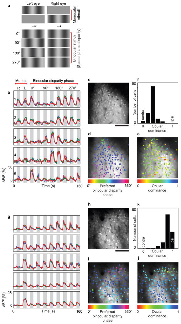
Figure 1
Single-cell responses and functional maps from two experiments. a , Monocular and binocular stimuli used to obtain maps for ocular dominance and binocular disparity, respectively. Arrows pointing in t...
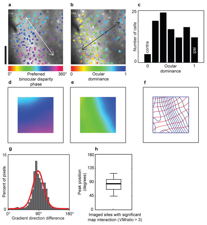
Figure 2
Orthogonal maps for binocular disparity and ocular dominance when gradients were evident in both maps. au2013b , Disparity and ocular dominance cell-based maps from a single imaged site 204 u03bcm bel...
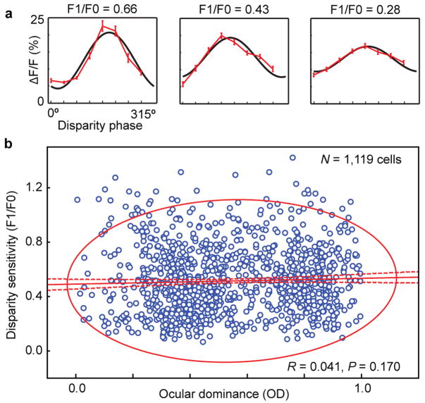
Figure 3
Relationship between disparity sensitivity and the response to monocular stimuli. a , Disparity tuning curve for three cells. Data are shown in red, mean u00b1 s.e.m, for the eight disparities present...
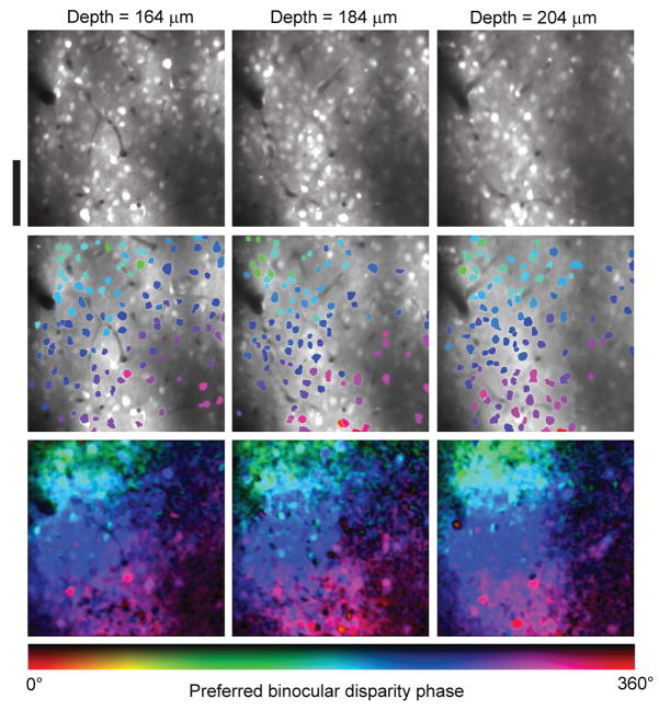
Figure 4
Stable functional micro-architecture for binocular disparity. Anatomical images 300 u00d7 300 u03bcm (top row), cell-based disparity phase maps (middle row), and pixel-based disparity phase maps (bott...
Figure images are served from the NIH/NLM PubMed Central Open Access Subset or Europe PMC; copyright remains with the publishers and authors.
💬 Discussion
0 commentsNo comments yet. Be the first to start a discussion!
Leave a Comment