Abstract
We present Skan (Skeleton analysis), a Python library for the analysis of the skeleton structures of objects. It was inspired by the "analyse skeletons" plugin for the Fiji image analysis software, but its extensive Application Programming Interface (API) allows users to examine and manipulate any intermediate data structures produced during the analysis. Further, its use of common Python data structures such as SciPy sparse matrices and pandas data frames opens the results to analysis within the extensive ecosystem of scientific libraries available in Python. We demonstrate the validity of Skan's measurements by comparing its output to the established Analyze Skeletons Fiji plugin, and, with a new scanning electron microscopy (SEM)-based method, we confirm that the malaria parasite Plasmodium falciparum remodels the host red blood cell cytoskeleton, increasing the average distance between spectrin-actin junctions.
🔬 Techniques
🧬 Organisms
🧪 Sample Preparation
💻 Software Details
💻 Code & Software
💾 Data Repositories
🏛️ Research Organizations (ROR)
Affiliated research institutions:
📋 Methods
Analysis of skeleton model from DIADEM challenge
We downloaded the olfactory projection neuron 1 (OP-1) model as a SWC file from DIADEM’s website at http://diademchallenge.org/data_set_downloads.html , along with its corresponding 3D TIFF image stack. We then rasterised the model (i.e., converted it from a network of vertex coordinates to a set of active pixels) by using the Simple Neurite Tracer ( Longair, Baker & Armstrong, 2011 ) plugin for Fiji, function “Analysis > Render/Analyze Skeletonized Paths.” This produces a 6-connected skeleton path, which we needed to convert to a (thinner) 26-connected path, so we further skeletonized the raster with the morphology.skeletonize3d function from scikit-image ( Van der Walt et al., 2014 ), and saved it as a compressed TIFF file. Then, we imported this raster image into either Fiji or Python (using Christoph Gohlke’s TIFF file). In both cases, we manually set the scale to 9.100602 × 3.033534 × 3.033534 μm per voxel, as documented on the DIADEM website. In Fiji, we used “Analyze Skeletons” with the “Show detailed info” option ticked, saved the results to csv, and loaded them into a pandas DataFrame in Python. In Python, we used skan.csr.summarise to produce a corresponding pandas DataFrame for Skan’s analysis. Finally, we used numpy.histogram and matplotlib.pyplot.hist ( Hunter, 2007 ) to produce the histogram in Fig. 1 . 10.7717/peerj.4312/fig-1 Figure 1 Comparison of skan and Fiji analysis results of the neuronal skeleton from olfactory projection neuron 1 (OP-1) from the DIADEM challenge. (A) Depth projection of the neuron. Scale bar: 500 μm. Colour map: height in μm. (B) Skeleton of the neuron. (C) Distribution of 82 branch lengths between 103 branch points measured by Skan and Fiji in the neuronal skeleton. (D) Distance from 103 skan junction points to the nearest Fiji junction point. Note that the voxel spacing is approximately 9 × 3 × 3 μm, so almost all of these distances are less than one pixel apart.
Show full methods section
Analysis of skeleton model from DIADEM challenge
We downloaded the olfactory projection neuron 1 (OP-1) model as a SWC file from DIADEM’s website at http://diademchallenge.org/data_set_downloads.html , along with its corresponding 3D TIFF image stack. We then rasterised the model (i.e., converted it from a network of vertex coordinates to a set of active pixels) by using the Simple Neurite Tracer ( Longair, Baker & Armstrong, 2011 ) plugin for Fiji, function “Analysis > Render/Analyze Skeletonized Paths.” This produces a 6-connected skeleton path, which we needed to convert to a (thinner) 26-connected path, so we further skeletonized the raster with the morphology.skeletonize3d function from scikit-image ( Van der Walt et al., 2014 ), and saved it as a compressed TIFF file. Then, we imported this raster image into either Fiji or Python (using Christoph Gohlke’s TIFF file). In both cases, we manually set the scale to 9.100602 × 3.033534 × 3.033534 μm per voxel, as documented on the DIADEM website. In Fiji, we used “Analyze Skeletons” with the “Show detailed info” option ticked, saved the results to csv, and loaded them into a pandas DataFrame in Python. In Python, we used skan.csr.summarise to produce a corresponding pandas DataFrame for Skan’s analysis. Finally, we used numpy.histogram and matplotlib.pyplot.hist ( Hunter, 2007 ) to produce the histogram in Fig. 1 . 10.7717/peerj.4312/fig-1 Figure 1 Comparison of skan and Fiji analysis results of the neuronal skeleton from olfactory projection neuron 1 (OP-1) from the DIADEM challenge. (A) Depth projection of the neuron. Scale bar: 500 μm. Colour map: height in μm. (B) Skeleton of the neuron. (C) Distribution of 82 branch lengths between 103 branch points measured by Skan and Fiji in the neuronal skeleton. (D) Distance from 103 skan junction points to the nearest Fiji junction point. Note that the voxel spacing is approximately 9 × 3 × 3 μm, so almost all of these distances are less than one pixel apart.
Tissue origin and ethics approval
This study made use of donated human red blood cells. All experiments were approved by The University of Melbourne School of Biomedical Sciences, Human Ethics Advisory Group (HEAG), for project titled “Characterising host cell interactions in the human malaria parasite, Plasmodium falciparum”, and ethics ID 1135799. Cells were obtained by a Material Supply Agreement with the Australian Red Cross Blood Service, agreement number—17-05VIC-23.
Sample preparation and SEM imaging
To prepare sheared membranes, infected and uninfected red blood cells were attached to 3-Aminopropyl-triethoxysilane treated glass slides using the lectin erythro-agglutinating phytohemagglutinin (PHA-E) and sheared in a hypotonic buffer according to a previously established procedure ( Shi et al., 2013 ). Sheared membranes were immediately fixed with 2.5% glutaraldehyde for 1 h before dehydration in a series of ethanol:water mixtures of 20, 50, 70, 80, 90, 95 and (3×) 100% ethanol for 5 min each and finally being allowed to dry in air. Dried samples were gold coated on the rotating mount of a Dynavac SC100 sputter coating instrument for 35 s using a 25 mA current, measuring 0.2 nm thickness on the quartz crystal microbalance. The coating procedure was optimised to prevent under- or overcoating which presents problems with the skeleton trace. SEM images were recorded using the ETD detector (in Optiplan mode) of an FEI Teneo instrument with a working distance of 5 mm, a beam current of 50 pA and a 2 kV accelerating voltage. Multiple images at 200–250 k magnification were recorded per individual cell to cover a greater portion of the membrane. Extraction of skeleton data from SEM images In our SEM images, the spectrin-actin network appears as bright (raised) patches over dark patches of background (see Fig. 1 ). We followed a simple approach to trace the midline of the spectrin branches: smoothing the images, then thresholding them ( Sauvola & Pietikäinen, 2000 ), and finally thinning them ( Zhang & Suen, 1984 ). The width of the Gaussian smoothing, the window size for thresholding, and the offset for the thresholding are all parameters of our approach, and are recorded in the results output file of a skeleton analysis (when using the graphical user interface).
Data and code availability
Our code is open source and available at https://github.com/jni/skan . Its documentation can be viewed at https://jni.github.io/skan and includes all code necessary to reproduce Fig. 2 . Additional scripts used in our analyses are available at https://github.com/jni/skan-scripts . 10.7717/peerj.4312/fig-2 Figure 2 Infection by the malaria parasite remodels the spectrin skeleton of the host red blood cell in the asexual developmental stage. (A) Example image produced by our protocol. Scale bar: 300 nm. (B) Thresholding (white) and skeletonisation (red) of the image in (A). (C) Complete distribution of measured spectrin branch lengths for normal and infected RBCs. (D) Mean spectrin branch length by cell ( n norm = 10, n inf = 13). We have made the schizont SEM dataset available at the Open Science Framework (OSF), with DOI 10.17605/OSF.IO/SVPFU , together with an archive of the documentation at time of publication, and a sample Excel file resulting from analysing the schizont dataset using the GUI.
Supplemental Information 10.7717/peerj.4312/supp-1 Figure S1 Strategies for resolving skeleton junctions (A) A minimal skeleton. (B) Skan’s classification of pixels into endpoints, paths, and junctions based on the number of neighbours (1, 2, and 3 or more, respectively). (C) Identical classification in Fiji’s Analyze Skeletons. (D) Skeleton measurement when junctions are assigned an implicit “extent”. (E) Skeleton measurement when all adjacent junction pixels are replaced by their centroid (our default strategy). (F) Skeleton measurement used in Fiji’s Analyze skeletons (mid-2017 version). Click here for additional data file. 10.7717/peerj.4312/supp-2 Supplemental Information 2 Supplementary results Pixel-level comparison with Analyze Skeletons. Click here for additional data file.
📊 Figures
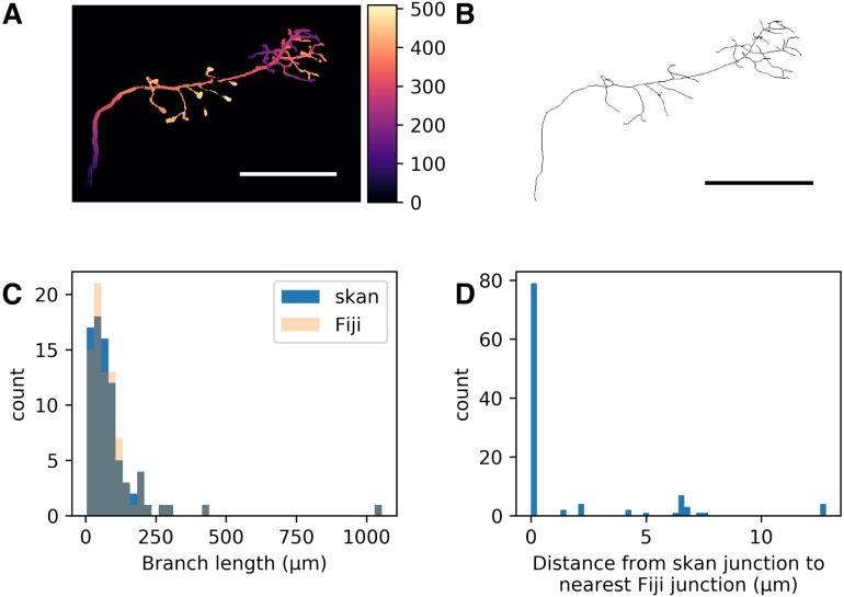
Figure 1
Comparison of skan and Fiji analysis results of the neuronal skeleton from olfactory projection neuron 1 (OP-1) from the DIADEM challenge.
(A) Depth projection of the neuron. Scale bar: 500u00a0u03bcm. Colour map: height in u03bcm. (B) Skeleton of the neuron. (C) Distribution of 82 branch lengths between 103 branch points measured by Ska...
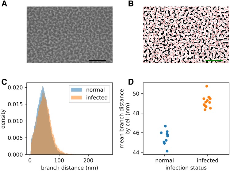
Figure 2
Infection by the malaria parasite remodels the spectrin skeleton of the host red blood cell in the asexual developmental stage.
(A) Example image produced by our protocol. Scale bar: 300 nm. (B) Thresholding (white) and skeletonisation (red) of the image in (A). (C) Complete distribution of measured spectrin branch lengths for...
Figure images are served from the NIH/NLM PubMed Central Open Access Subset or Europe PMC; copyright remains with the publishers and authors.
💬 Discussion
0 commentsNo comments yet. Be the first to start a discussion!
Leave a Comment