Abstract
AbstractPsychological stress affects a wide spectrum of brain functions and poses risks for many mental disorders. However, effective therapeutics to alleviate or revert its deleterious effects are lacking. A recently synthesized psychedelic analog tabernanthalog (TBG) has demonstrated anti-addictive and antidepressant potential. Whether TBG can rescue stress-induced affective, sensory, and cognitive deficits, and how it may achieve such effects by modulating neural circuits, remain unknown. Here we show that in mice exposed to unpredictable mild stress (UMS), administration of a single dose of TBG decreases their anxiety level and rescues deficits in sensory processing as well as in cognitive flexibility. Post-stress TBG treatment promotes the regrowth of excitatory neuron dendritic spines lost during UMS, decreases the baseline neuronal activity, and enhances whisking-modulation of neuronal activity in the somatosensory cortex. Moreover, calcium imaging in head-fixed mice performing a whisker-dependent texture discrimination task shows that novel textures elicit responses from a greater proportion of neurons in the somatosensory cortex than do familiar textures. Such differential response is diminished by UMS and is restored by TBG. Together, our study reveals the effects of UMS on cortical neuronal circuit activity patterns and demonstrate that TBG combats the detrimental effects of stress by modulating basal and stimulus-dependent neural activity in cortical networks.
🔬 Techniques
🔭 Microscopes
💻 Software
✨ Fluorophores
🧪 Sample Preparation
🏭 Microscope Brands
🧪 Reagent Suppliers
🔴 Lasers
🎨 Filters
💻 Software Details
🏛️ Research Organizations (ROR)
Affiliated research institutions:
📋 Methods
Experimental animals Thy1 -GFP-M (JAX #007788) and C57BL/6J (JAX #000664) mice were purchased from the Jackson Laboratory. Mice were group-housed with littermates and maintained on a 12 h light/dark cycle. Both sexes of mice aged 1–2 months were used. Unless otherwise noted, all experiments were carried out on C57BL/6J mice. Mice were randomly assigned to experimental groups. All animal experiments were carried out in accordance with protocols approved by the IACUC of University of California Santa Cruz or by Stanford University Administrative Panel on Laboratory Animal Care. Unpredictable mild stress We subjected 2-month old mice to 7-day UMS as previously described [ 38 ]. Briefly, the mice were exposed to mild stressors as listed in Supplementary Table 1 . Elevated plus maze (EPM) EPM test was performed according to established protocols [ 39 ] with slight modifications. We used a custom-made plexiglass EPM. The four arms were 30 cm × 5 cm (L × H); the two closed arms were enclosed by walls 15 cm in height. The apparatus was elevated 50 cm from the ground by sturdy metal posts. Each mouse was allowed to explore the EPM freely for 5 min. Mouse behavior was monitored with a video-tracking system controlled by Bonsai [ 40 ]. We used DeepLabCut [ 41 ] to track multiple points on the mouse (nose, head, neck, body, and base of the tail) through all video frames, and used custom-written Python 3.6 and Matlab R2019a (MathWorks, Natick, MA) programs to quantify the total distance traveled and the time spent in open vs. closed arms, based on the location of the body point. Four-choice odor discrimination and reversal We followed the protocol described previously [ 42 ] with slight modifications. The four-chamber arena is a 12” × 12” × 9” (L × W × H) box constructed of 0.25” white acrylic, with 4 quadrants partially divided by 3”-wide internal walls made of transparent acrylic. White ceramic ramekins (diameter = 2.88”, depth = 1.75”) were used to present odor stimuli and food reward. The odor stimuli were essential oils (rosemary, clove, thyme, nutmeg, or cinnamon; LorAnn Oils, Lansing, MI). Food rewards were small pieces (~10 mg each) of Honey Nut Cheerio (General Mills, Minneapolis, MN). Digging media were made of pine shavings (Grreat Choice®, www.petsmart.com). Between trials, the mouse was confined by a removable transparent acrylic cylinder (diameter = 6”) in the center of the arena. The arena was wiped with 70% ethanol between animals. The mouse was food restricted starting ~5 days before the testing day so that its body weight was reduced to 80–85% of the baseline. Meanwhile it was also handled 10 min daily for 3 days, followed by a two-day pre-training procedure before the testing day. On pre-training day 1 (acclimation), the mouse was habituated to the arena and the ramekins (one in each quadrant) for 1 h. Food rewards were placed in all ramekins without digging medium coverage. On pre-training day 2 (shaping), the mouse learned to dig in the media to find buried food reward. Only one ramekin was used in this phase, and the quadrant containing it was rotated between trials (SE to NW to SW to NE), with all quadrants rewarded equally. In the first 4 trials, the cereal piece was not covered with wood shaving. Over the next trials the amount of wood shavings gradually increased, from a dusting of shavings (4 trials) to quarter full (4 trials), half full (4 trials), and finally to full coverage of the cereal piece (12 trials). Trials were untimed, and most mice completed shaping within 1 h. On the testing day, the mouse was subjected to a four-choice discrimination session followed by a reversal session. Each quadrant of the arena contained one ramekin filled with wood shavings and scented by applying a drop of essential oil onto a small piece of filter paper affixed to the ramekin wall. During the initial discrimination phase, the mouse discriminated among the four odors (rosemary, clove, thyme, and nutmeg) and learned which one was associated with the buried cereal reward. The placement of ramekins was pseudo-randomized such that the same odor was not presented in the same quadrant over two consecutive trials. In each trial, the mouse could freely explore the arena until it started digging in a ramekin (rather than merely sniffing or chewing the shavings). If the mouse made a correct choice, the trial was terminated after it finished eating the food reward; if it made an incorrect choice the trial was terminated after it finished digging. If the mouse did not make any choice within 3 min, the trial was terminated and recorded as an “omission”. After each trial, the mouse was returned to the arena center with cylinder confinement, and ramekins were rearranged and re-baited if necessary. The session criterion was met if the mouse correctly completed 8 out of 10 consecutive trials. The mouse moved on to the reversal session immediately after passing the discrimination session. All shavings were replaced with fresh shavings, and thyme was swapped out for a novel odor, cinnamon. The session criterion was the same as above. Whisker-dependent texture discrimination (WTD) The WTD test on free-moving mice was performed as previously described [ 15 , 43 ]. Prior to testing, the subject mouse was habituated to the testing chamber (L × W × H = 38 cm × 28 cm × 23 cm) for 10 min per day for 2 days. On the testing day, the mouse went through habituation (3 min), encoding (5 min), resting (5 min), and testing (3 min). During encoding, the mouse was presented with two columns (3 cm × 3 cm × 12 cm) coated with the same texture (e.g., 220 grit sandpaper). During testing the columns were replaced with a new pair, one with the same texture as before (familiar) and the other with a novel texture (e.g., 60 grit sandpaper), for the mouse to explore. We excluded mice showing insufficient interest in the columns (i.e., 60% approaching time spent on one column) during encoding from further testing. The WTD test on head-fixed mice was performed using the Neurotar mobile home cage (MHC; Neurotar Oy Ltd, Helsinki, Finland). The mouse was handled 5–10 min per day for 3 days to habituate it to the experimenter. Then the mouse was habituated to head-fixation on the empty MHC (1 h session × 2 per day for at least 6 days). On the testing day the mouse went through 4 phases: free exploration (5 min), encoding (15 min), resting (10 min), and testing (15 min). During encoding, the mouse was presented with two identical textures (e.g., 5 cm × 5 cm patches of 220 grit sandpaper attached to the MHC wall, separated by 90 degrees) to explore. During resting, the textures were removed and the mouse was allowed to rest or explore the empty MHC at will. During testing, two fresh textures were attached to the MHC wall, one identical to the texture previously presented, the other novel (e.g., 60 grit sandpaper). Mouse behavior was recorded with an infrared camera (Cameleon 3 monochrome CM3-U3-13Y3M-CS, FLIR Systems, Inc., Richmond, BC, Canada) and analyzed offline using the Boris program [ 44 ]. We quantified the number of approaches and the amount of time spent actively investigating the columns, and computed the discrimination index (DI) as follows: documentclass[12pt]{minimal} usepackage{amsmath} usepackage{wasysym} usepackage{amsfonts} usepackage{amssymb} usepackage{amsbsy} usepackage{mathrsfs} usepackage{upgreek} setlength{oddsidemargin}{-69pt} begin{document}$${it{DI}} = frac{{{mathrm{approaches}},{mathrm{to}},{mathrm{novel}},{mathrm{texture}} - {mathrm{approaches}},{mathrm{to}},{mathrm{familiar}},{mathrm{texture}}}}{{{mathrm{approaches}},{mathrm{to}},{mathrm{both}},{mathrm{textures}}}}$$end{document} D I = approaches to novel texture − approaches to familiar texture approaches to both textures Drug preparation and administration TBG was synthesized in the lab of David E. Olson as described previously [ 36 ]. TBG or fluoxetine hydrochloride (Cat #0927-10, Tocris Bioscience, Bristol, U.K.) was administered to the mouse intraperitoneally (i.p.) at a dosage of 10 mg/kg of bodyweight. USP-grade saline (0.9%) was used as vehicle.
Show full methods section
Experimental animals Thy1 -GFP-M (JAX #007788) and C57BL/6J (JAX #000664) mice were purchased from the Jackson Laboratory. Mice were group-housed with littermates and maintained on a 12 h light/dark cycle. Both sexes of mice aged 1–2 months were used. Unless otherwise noted, all experiments were carried out on C57BL/6J mice. Mice were randomly assigned to experimental groups. All animal experiments were carried out in accordance with protocols approved by the IACUC of University of California Santa Cruz or by Stanford University Administrative Panel on Laboratory Animal Care. Unpredictable mild stress We subjected 2-month old mice to 7-day UMS as previously described [ 38 ]. Briefly, the mice were exposed to mild stressors as listed in Supplementary Table 1 . Elevated plus maze (EPM) EPM test was performed according to established protocols [ 39 ] with slight modifications. We used a custom-made plexiglass EPM. The four arms were 30 cm × 5 cm (L × H); the two closed arms were enclosed by walls 15 cm in height. The apparatus was elevated 50 cm from the ground by sturdy metal posts. Each mouse was allowed to explore the EPM freely for 5 min. Mouse behavior was monitored with a video-tracking system controlled by Bonsai [ 40 ]. We used DeepLabCut [ 41 ] to track multiple points on the mouse (nose, head, neck, body, and base of the tail) through all video frames, and used custom-written Python 3.6 and Matlab R2019a (MathWorks, Natick, MA) programs to quantify the total distance traveled and the time spent in open vs. closed arms, based on the location of the body point. Four-choice odor discrimination and reversal We followed the protocol described previously [ 42 ] with slight modifications. The four-chamber arena is a 12” × 12” × 9” (L × W × H) box constructed of 0.25” white acrylic, with 4 quadrants partially divided by 3”-wide internal walls made of transparent acrylic. White ceramic ramekins (diameter = 2.88”, depth = 1.75”) were used to present odor stimuli and food reward. The odor stimuli were essential oils (rosemary, clove, thyme, nutmeg, or cinnamon; LorAnn Oils, Lansing, MI). Food rewards were small pieces (~10 mg each) of Honey Nut Cheerio (General Mills, Minneapolis, MN). Digging media were made of pine shavings (Grreat Choice®, www.petsmart.com). Between trials, the mouse was confined by a removable transparent acrylic cylinder (diameter = 6”) in the center of the arena. The arena was wiped with 70% ethanol between animals. The mouse was food restricted starting ~5 days before the testing day so that its body weight was reduced to 80–85% of the baseline. Meanwhile it was also handled 10 min daily for 3 days, followed by a two-day pre-training procedure before the testing day. On pre-training day 1 (acclimation), the mouse was habituated to the arena and the ramekins (one in each quadrant) for 1 h. Food rewards were placed in all ramekins without digging medium coverage. On pre-training day 2 (shaping), the mouse learned to dig in the media to find buried food reward. Only one ramekin was used in this phase, and the quadrant containing it was rotated between trials (SE to NW to SW to NE), with all quadrants rewarded equally. In the first 4 trials, the cereal piece was not covered with wood shaving. Over the next trials the amount of wood shavings gradually increased, from a dusting of shavings (4 trials) to quarter full (4 trials), half full (4 trials), and finally to full coverage of the cereal piece (12 trials). Trials were untimed, and most mice completed shaping within 1 h. On the testing day, the mouse was subjected to a four-choice discrimination session followed by a reversal session. Each quadrant of the arena contained one ramekin filled with wood shavings and scented by applying a drop of essential oil onto a small piece of filter paper affixed to the ramekin wall. During the initial discrimination phase, the mouse discriminated among the four odors (rosemary, clove, thyme, and nutmeg) and learned which one was associated with the buried cereal reward. The placement of ramekins was pseudo-randomized such that the same odor was not presented in the same quadrant over two consecutive trials. In each trial, the mouse could freely explore the arena until it started digging in a ramekin (rather than merely sniffing or chewing the shavings). If the mouse made a correct choice, the trial was terminated after it finished eating the food reward; if it made an incorrect choice the trial was terminated after it finished digging. If the mouse did not make any choice within 3 min, the trial was terminated and recorded as an “omission”. After each trial, the mouse was returned to the arena center with cylinder confinement, and ramekins were rearranged and re-baited if necessary. The session criterion was met if the mouse correctly completed 8 out of 10 consecutive trials. The mouse moved on to the reversal session immediately after passing the discrimination session. All shavings were replaced with fresh shavings, and thyme was swapped out for a novel odor, cinnamon. The session criterion was the same as above. Whisker-dependent texture discrimination (WTD) The WTD test on free-moving mice was performed as previously described [ 15 , 43 ]. Prior to testing, the subject mouse was habituated to the testing chamber (L × W × H = 38 cm × 28 cm × 23 cm) for 10 min per day for 2 days. On the testing day, the mouse went through habituation (3 min), encoding (5 min), resting (5 min), and testing (3 min). During encoding, the mouse was presented with two columns (3 cm × 3 cm × 12 cm) coated with the same texture (e.g., 220 grit sandpaper). During testing the columns were replaced with a new pair, one with the same texture as before (familiar) and the other with a novel texture (e.g., 60 grit sandpaper), for the mouse to explore. We excluded mice showing insufficient interest in the columns (i.e., 60% approaching time spent on one column) during encoding from further testing. The WTD test on head-fixed mice was performed using the Neurotar mobile home cage (MHC; Neurotar Oy Ltd, Helsinki, Finland). The mouse was handled 5–10 min per day for 3 days to habituate it to the experimenter. Then the mouse was habituated to head-fixation on the empty MHC (1 h session × 2 per day for at least 6 days). On the testing day the mouse went through 4 phases: free exploration (5 min), encoding (15 min), resting (10 min), and testing (15 min). During encoding, the mouse was presented with two identical textures (e.g., 5 cm × 5 cm patches of 220 grit sandpaper attached to the MHC wall, separated by 90 degrees) to explore. During resting, the textures were removed and the mouse was allowed to rest or explore the empty MHC at will. During testing, two fresh textures were attached to the MHC wall, one identical to the texture previously presented, the other novel (e.g., 60 grit sandpaper). Mouse behavior was recorded with an infrared camera (Cameleon 3 monochrome CM3-U3-13Y3M-CS, FLIR Systems, Inc., Richmond, BC, Canada) and analyzed offline using the Boris program [ 44 ]. We quantified the number of approaches and the amount of time spent actively investigating the columns, and computed the discrimination index (DI) as follows: documentclass[12pt]{minimal} usepackage{amsmath} usepackage{wasysym} usepackage{amsfonts} usepackage{amssymb} usepackage{amsbsy} usepackage{mathrsfs} usepackage{upgreek} setlength{oddsidemargin}{-69pt} begin{document}$${it{DI}} = frac{{{mathrm{approaches}},{mathrm{to}},{mathrm{novel}},{mathrm{texture}} - {mathrm{approaches}},{mathrm{to}},{mathrm{familiar}},{mathrm{texture}}}}{{{mathrm{approaches}},{mathrm{to}},{mathrm{both}},{mathrm{textures}}}}$$end{document} D I = approaches to novel texture − approaches to familiar texture approaches to both textures Drug preparation and administration TBG was synthesized in the lab of David E. Olson as described previously [ 36 ]. TBG or fluoxetine hydrochloride (Cat #0927-10, Tocris Bioscience, Bristol, U.K.) was administered to the mouse intraperitoneally (i.p.) at a dosage of 10 mg/kg of bodyweight. USP-grade saline (0.9%) was used as vehicle.
Cranial window implantation and virus injection
We performed cranial window implantation and virus injection on mice around postnatal day (P)30 according to established protocols [ 45 ] with slight modifications. In brief, the mouse was anesthetized with isoflurane (4% for induction, 1.5% for maintenance). Ophthalmic ointment was applied to prevent eye desiccation and irritation; dexamethasone (2 μg/g bodyweight) was injected into the quadriceps, and carprofen (5 μg/g bodyweight) was injected intraperitoneally. A circular piece of the skull was removed with a trephine (diameter = 2.3 mm, Fine Science Tools, Foster City, CA) driven by a high-speed micro-drill (Foredom K1070, Blackstone Industries, LLC, Bethel, CT). The window centered at AP = −1.5 mm, ML = 3.5 mm for barrel cortex (S1BF), or AP = +1.7 mm, ML = 1.0 mm for frontal cortex. For dendritic spine imaging, we used the thy1 -GFP-M line mice, which express cytoplasmic GFP in a sparse subset of cortical neurons [ 46 ]. For Ca imaging of cortical L2/3 neurons, we used C57BL/6J mice and injected AAV2/1-Syn-GCaMP6f-WPRE-SV40 (Addgene 100837-AAV1) at two sites (~150 nl per site) near the center of the cranial window using a custom-built injection system based on a single-axis oil hydraulic micromanipulator (Narishige, Tokyo, Japan), targeting 150–200 μm below pial surface. The cranial window was sealed with an imaging port made of a round glass coverslip (#1, diameter = 2.3 mm) glued to an overlaying annular glass “doughnut” (#1, inner diameter = 2 mm, outer diameter = 3 mm, Potomac Photonics, Inc., Baltimore, MD). Dental cement (Jet Denture Repair, Lang Dental, Wheeling, IL) was applied over the exposed skull to secure a custom-made stainless-steel head plate onto the skull. The mouse received the antibiotic enrofloxacin (5 μg/g bodyweight) and the analgesic buprenorphine (0.1 μg/g bodyweight) preemptively and then daily for 2 more days. In vivo spine imaging and image analysis In vivo two-photon (2P) imaging of dendritic spines was performed on a 2P microscope (Ultima Investigator, Bruker Co., Middleton, WI) equipped with a 16× NA = 0.8 water immersion objective (CFI75 LWD 16X W, Nikon Instruments, Inc., Melville, NY) and an ultrafast 2P laser (Mai Tai, Spectra-Physics, Santa Clara, CA) operating at 940 nm. The mouse was anaesthetized with an intraperitoneal injection of a mixture of 17 mg/ml ketamine and 1.7 mg/ml xylazine in 0.9% saline (5.0 ml/kg bodyweight), and mounted on a custom-made stage for imaging. Stacks of images were acquired with a Z-step size of 1 µm at 12× zoom. Relocation of the same dendrites in subsequent imaging sessions was achieved by reference to blood vessels and the dendritic branching pattern. Data analysis was performed in ImageJ as described previously [ 47 , 48 ]. Typically, 150–200 spines were analyzed per animal per session. The percentage of spines formed/eliminated was calculated as the number of spines formed/eliminated divided by the total number of spines counted from the previous imaging session. Morphological categorization of spines was performed according to criteria described previously [ 49 ]. Filopodia were identified as described previously [ 50 ]. The percentage of filopodia formed/eliminated was calculated as the number of filopodia formed/eliminated divided by the total number of protrusions (spines plus filopodia) counted from the previous imaging session. In vivo wide-field Ca imaging and image analysis The awake mouse was head-fixed over a custom-made flat rotating disk on which it may run or rest at will. Wide-field Ca imaging through the cranial window was performed on a custom-built mesoscope adapted from a previously published design [ 51 ] (see Fig. 3a for a schematic drawing). Briefly, images of the brain surface were taken through a pair of photographic lenses in tandem (focal length 50 mm, F = 1.2 and 5.6, respectively) coupled to a scientific cMOS camera (PCO Edge 5.5, ~6.5 μm pixel resolution; PCO AG, Kelheim, Germany). A blue light-emitting diode (470 nm, max power 1000 mW; Thorlabs #M470L3) provides the excitation light, which passes through a 480/30 nm bandpass filter (Chroma Technology AT480/30x) and is deflected by a dichroic mirror (Chroma Technology T4951pxr). Emitted fluorescence passes through a 520/36 nm bandpass filter (Edmund Optics 67-044) and is detected by the camera. In each imaging session, 16-bit images (400 × 400 pixels) were collected at 10 frames per second (fps) for 15 min. A profile view of the mouse, focusing on the whisker pad contralateral to the cranial window, was collected concurrently with an infrared camera (Raspberry Pi NoIR V2) at 30 fps triggered by the onset of wide-field imaging. Wide-field Ca imaging data were first processed with pySEAS, an independent component analysis (ICA) filtering method to remove components corresponding to hemodynamic changes; other components were recombined for subsequent data analysis [ 52 ]. A mask for the regions with strong virus expression was generating by thresholding the autocorrelation of dF/F 0 of each pixel (threshold = 0.95). Only pixels in the masked regions were used for subsequent analysis. To define whisking episodes, we first manually selected a region of interest (ROI) around the whisker pad from the behavioral video in OpenCV. We then used a grid-based optic flow algorithm to calculate the motion magnitude across grid points. We used the average motion magnitude of all grid points to represent the magnitude of whisking. The whole-field Ca activity Ca WF was defined as the average dF/F 0 over all pixels in the masked region. Its cross-correlation with whisking magnitude was defined with the Pearson correlation coefficient calculated in Python 3.6 using the NumPy function numpy_correlate . For trial-by-trial analysis, Ca WF around the onset of each whisking episode (−2 s to +2 s) were extracted and aligned. The whisking-modulation of Ca WF was calculated as follows: first subtract the average pre-onset Ca WF over (−1 s to 0 s) from the average post-onset Ca WF over (0.3 s to 1.3 s) for each episode, then average the results over all whisking episodes for each animal. The response window was chosen based on a previous work [ 53 ]. The response delay was calculated as follows: first find the maximum value of post-onset Ca WF over (0.3 s to 1.3 s) for each episode, then average the results over all whisking episodes for each animal. The cross-correlation between whisking magnitude and individual pixel’s dF/F 0 was computed using the NumPy library as above. In vivo 2P Ca imaging and image analysis Imaging was performed with a 2P microscope (Ultima Investigator, Bruker Co., Middleton, WI) equipped with a 16× NA = 0.8 water immersion objective (CFI75 LWD 16X W, Nikon Instruments, Inc., Melville, NY), a resonant scanner, and an ultrafast 2P laser (Mai Tai, Spectra-Physics, Santa Clara, CA) operating at 940 nm. Ca images (512 × 512 pixels) were taken at 150–200 μm beneath the pial surface at 30 fps. Image series were motion-corrected with the “moco” plug-in of ImageJ [ 54 ] and then down-sampled to 10 fps by average every three consecutive images. ROIs corresponding to individual neurons were manually delineated from the standard deviation projection image (along the time axis of the series) using ImageJ, and the mean pixel value F for each ROI was extracted. The extracted neuronal Ca traces were analyzed using a custom-written program in Matlab. According to the cell morphology and the appearance of Ca traces, the majority of neurons labeled by AAV2/1-Syn-GCaMP6f-WPRE-SV40 were excitatory, consistent with previously published observations [ 55 ]. Putative excitatory neurons with noisy signals and no apparent Ca transient were excluded from further analysis. To compute dF/F 0 , F 0 was estimated as the 50th percentile value of F within a 300 s sliding window. Ca transients and their peaks were detected using the Matlab function peakfinder , with minimal peak height = 4 × standard deviation of baseline dF/F 0 , minimal inter-peak interval = 0.5 s, and minimal transient width = 0.3 s. The denoised dF/F 0 was obtained by setting to zeros the values of the trace below 2 × standard deviation of baseline. Synchronous Ca events was detected and analyzed based on the previously published method [ 56 ] with slight modifications. Briefly, we first binarized each neuron’s denoised dF/F 0 by setting non-zero values to 1 and then summed the binarized Ca traces of all neurons to yield the population Ca trace. We then constructed surrogate population Ca traces (1000 trials) by circularly shuffling each neuron’s binarized Ca trace independently and summing the shuffled traces. The random circular shuffling maintains the average activity level of each neuron. We then found the 95th percentile value of all surrogate population Ca traces across the entire time course as the synchrony threshold. The time point at which the population Ca trace exceeded this threshold was set as the start of a synchronous Ca event, and the time point at which it fell below this threshold was set as the end of the event. A neuron was considered to participate in a synchronous event if it was active at the peak of the synchrony. To determine the pairwise correlation between neuronal Ca activities, we computed the Pearson correlation coefficient ρ between the dF/F 0 of each pair of neurons. In order to cluster neurons based on their pairwise correlation, we first transformed ρ into a distance metric documentclass[12pt]{minimal} usepackage{amsmath} usepackage{wasysym} usepackage{amsfonts} usepackage{amssymb} usepackage{amsbsy} usepackage{mathrsfs} usepackage{upgreek} setlength{oddsidemargin}{-69pt} begin{document}$$d = sqrt {(1 - rho )}$$end{document} d = ( 1 − ρ ) , and then constructed a hierarchical cluster tree based on this distance metric using the Matlab function linkage (with ‘complete’ method). We used the clustering results to order the neurons in the correlation matrix plot. We identified a “touch” event as the period of time lasting more than 1 s, during which whiskers contralateral to the imaged S1BF were in contact with the texture. We excluded shorter periods to ensure that the mouse was not merely passing by the texture unintentionally. The average touch response of a neuron to each texture was calculated as follows: first subtract the average baseline dF/F 0 (−1 s to 0 s before contact) from the average touch dF/F 0 (0.3 s to 1.3 s after interaction onset) for each interaction, then average the results over all interactions with the texture. We used receiver operating characteristic (ROC) analysis [ 57 ] to identify neurons responding to either novel or familiar texture, or both. We calculated the detection probability (DP), which is the probability with which an ideal observer could predict whether the Ca signal corresponds to a contact or baseline immediately before contact. To do so we split each episode of interaction into the pre-contact period (−1 s to 0 s) and the contact period (0.3 s to 1.3 s after contact onset), and assign the decision variable (DV) on the basis of the neuronal Ca activity (average dF/F 0 over the period). We then calculated DP as the area under the ROC curve for discrimination on the basis of DV. In order to assess the significance level, we performed a random permutation test, in which Ca activities during pre-contact and contact periods were randomly reshuffled (1000 times), and DP was calculated for each shuffling. We consider a neuron as responsive if p < 0.05. If a neuron responds exclusively to the novel or the familiar texture, it is classified as novel texture-selective (NTS) or familiar texture-selective (FTS), respectively. If a neuron responds to both textures, it is classified as non-selective. In vitro electrophysiology To prepare acute brain slices for patch-clamp recording [ 58 ], mice (aged 6–8 weeks) were anesthetized with isoflurane and decapitated. The brains were quickly removed and transferred into ice-cold cutting solution containing the following (in mM): 70 NaCl, 2.5 KCl, 1.25 NaH 2 PO 4 , 26 NaHCO 3 , 25 glucose, 75 sucrose, 4 MgCl 2 , and 0.5 CaCl 2 . 300 µm thick coronal slices were made with a vibratome (VT1200, Leica Microsystems, Wetzlar, Germany) in the cutting solution. After cutting, slices were immediately transferred to 32–34 °C artificial cerebrospinal fluid (ACSF) containing the following (in mM): 120 NaCl, 26 NaHCO 3 , 2.5 KCl, 11 glucose, 2 CaCl 2 , 2 MgSO 4 , and 1 NaH 2 PO 4 , (pH 7.3, ~300 mOsm). The ACSF and the cutting solution were balanced with 5% CO 2 / 95% O 2 . Slices recovered at 32–34 °C for 30 min before incubation in ACSF at room temperature. Patch-clamp recordings in the whole-cell configuration were performed at room temperature on PV+ INs in S1BF L2/3 (visualized with an Olympus BX51WI microscope). Recording pipettes (3–4 MΩ) were filled with the internal solution (in mM: 130 K-gluconate, 10 KCl, 10 HEPES, 5 MgATP, 0.3 Na 3 GTP, 0.2 EGTA, and 0.2% biocytin; pH 7.3, ~300 mOsm). For membrane property measurements, we broke-in under the voltage-clamp mode, held the cell at −70 mV, and immediately measured membrane resistance and capacitance. Once the cell was stabilized, we gradually reduced the holding current to 0, and then switched to current-clamp mode to measure resting membrane potential and other active membrane properties. The resting membrane potentials were recorded ~15 s after the switch to current-clamp mode. Input resistances were measured by holding the membrane potential at −60 mV. Action potential (AP) discharges and cell excitability were assessed by injections of a series of DC current steps (−50 to +330 pA in 20 pA increment for 800 ms, with 8 s inter-trial-interval) in the absence of any neurotransmitter receptor antagonist. The number of APs elicited by the injected currents was quantified. The rheobases were measured by injecting a series of current at 2 pA increment. Data were acquired using a Multiclamp 700B amplifier, Digidata 1440A, and pClamp10 software (Molecular Devices, San Jose, CA). Sampling rate was 20 kHz. Neurons with >10% changes in R m , R a , or C m were excluded from further analysis.
Quantifications and statistical analyses
Choice of sample size was based on studies published previously using similar animal models and experimental paradigms. All behavioral and imaging data were analyzed with the analyst blinded to the experimental conditions. All statistical analyses were performed with GraphPad Prism 8.4 (GraphPad Software, San Diego, CA). We performed the Shapiro–Wilk test for sample normality and examined the homogeneity of variance. Unless otherwise stated, if the sample met the assumptions for parametric tests, we used two-sided unpaired t -test for two-sample comparison, and one-way Analysis of Variance (ANOVA) followed by post hoc Tukey’s multiple comparisons for multi-sample comparison. If the sample failed to meet the assumptions for parametric tests, we used the Wilcoxon signed rank test for two-sample comparison, and the Kruskal–Wallis test followed by Dunn’s multiple comparisons for multi-sample comparison. We reported the sample sizes in the figures and the statistical tests used in the figure legends. We reported the p values of main effects in ANOVA or Kruskal–Wallis test in figure legends, and marked the p values of post hoc multiple comparisons in the figures with asterisks if they reached statistical significance (* p < 0.05, ** p < 0.01, *** p < 0.001, **** p < 1 × 10 –4 ); comparisons that did not reach statistical significance were not marked. Data are presented as mean ± s.e.m. unless otherwise stated.
Experimental animals Thy1 -GFP-M (JAX #007788) and C57BL/6J (JAX #000664) mice were purchased from the Jackson Laboratory. Mice were group-housed with littermates and maintained on a 12 h light/dark cycle. Both sexes of mice aged 1–2 months were used. Unless otherwise noted, all experiments were carried out on C57BL/6J mice. Mice were randomly assigned to experimental groups. All animal experiments were carried out in accordance with protocols approved by the IACUC of University of California Santa Cruz or by Stanford University Administrative Panel on Laboratory Animal Care.
Supplementary information Supplemental Material Supplemental Movie 1
📊 Figures
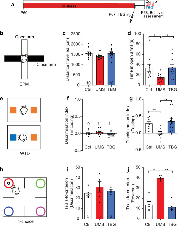
Fig. 1
TBG rescues UMS-induced behavioral deficits in mice.
a Timeline of UMS, drug injection, and behavioral tests. b Schematic of the elevated plus maze (EPM) test. c Total distance traveled in EPM ( H (3)u2009=u20094.437, p =u20090.1088, Kruskalu2013Wallis ...
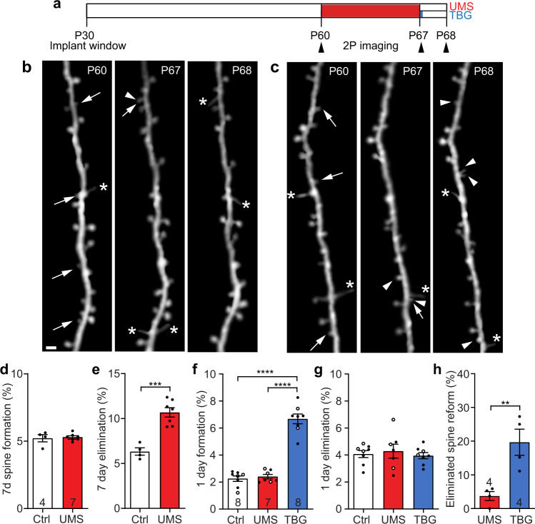
Fig. 2
TBG promotes spine formation that partially compensates for UMS-induced spine loss in the mouse cortex.
a Timeline of dendritic spine imaging experiments. b Example of the same set of S1BF spines imaged before UMS, immediately after UMS, and after 1-day recovery. c Example spine imaging over the same ti...
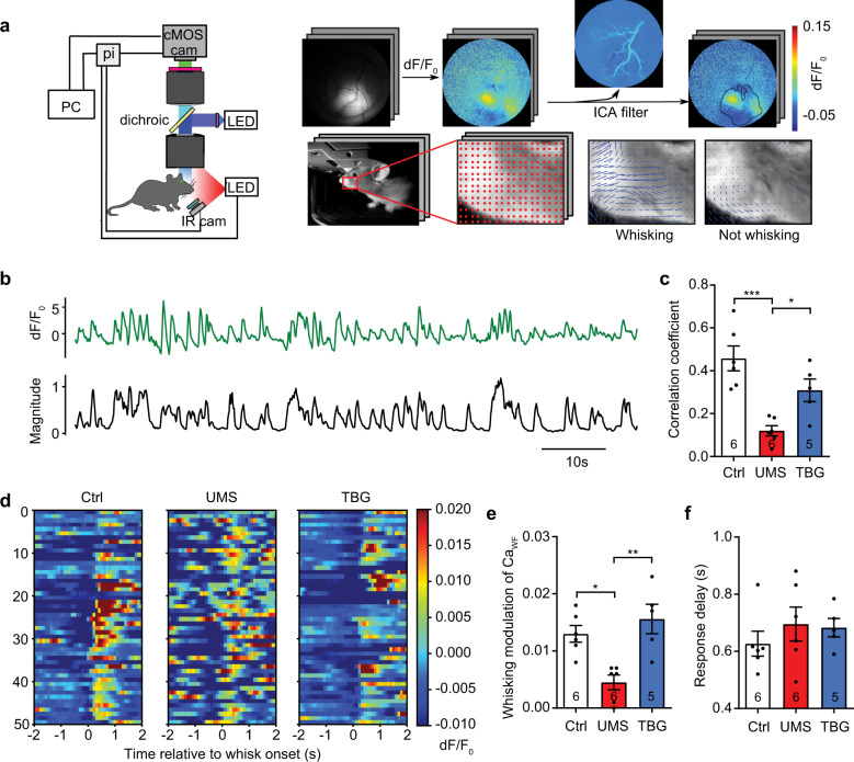
Fig. 3
TBG normalizes baseline and whisking-modulation of mesoscopic neural activities in S1BF following UMS.
a Schematic of mesoscope and data processing pipeline. pi: Raspberry Pi. Top: independent component analysis removes hemodynamic artifacts. Bottom: an optic flow algorithm identifies whisking episodes...
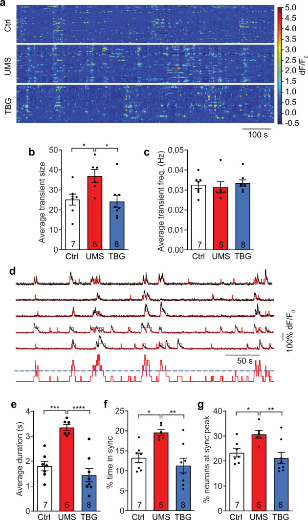
Fig. 4
TBG normalizes baseline Ca activities of S1BF L2/3 neurons following UMS.
a Example of baseline Ca activities of L2/3 neurons. b Average Ca transient size measured by the sum of dF/F 0 ( F (2,18)u2009=u20095.141, p <u20090.05, one-way ANOVA with post hoc Tukeyu2019s mult...
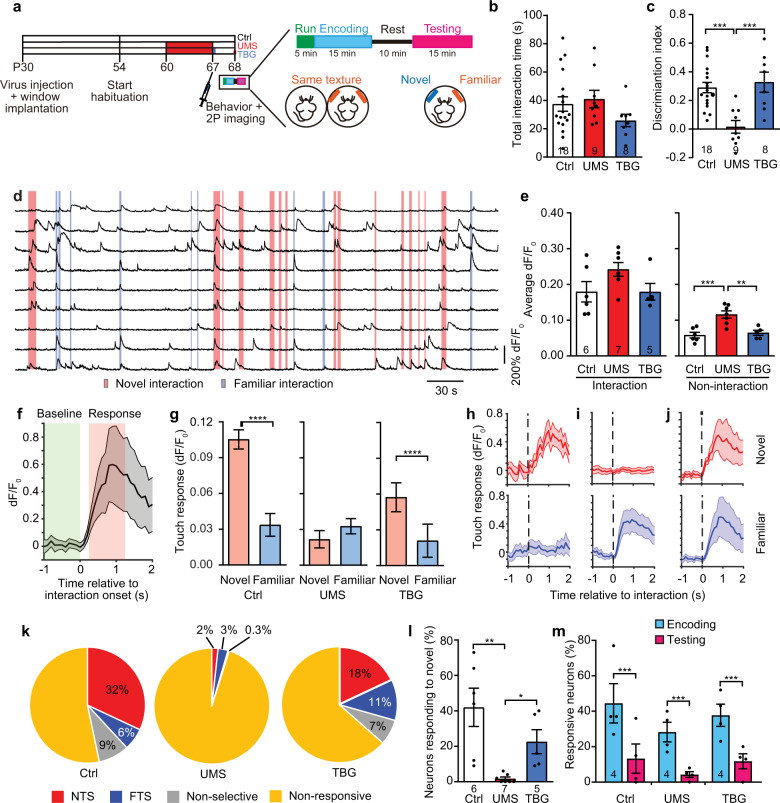
Fig. 5
Ca activity of S1BF L2/3 neurons during texture interaction was altered by UMS and rescued by TBG.
a Schematic of experimental design. b Total interaction time during testing ( F (2,32)u2009=u20091.487, p =u20090.2412, one-way ANOVA). c Discrimination index during testing ( F (2,32)u2009=u200910.95...
Figure images are served from the NIH/NLM PubMed Central Open Access Subset or Europe PMC; copyright remains with the publishers and authors.
💬 Discussion
0 commentsNo comments yet. Be the first to start a discussion!
Leave a Comment