Abstract
Bone histomorphometry allows quantitative evaluation of bone micro-architecture, bone formation, and bone remodeling by providing an insight to cellular changes. Histomorphometry plays an important role in monitoring changes in bone properties because of systemic skeletal diseases like osteoporosis and osteomalacia. Besides, quantitative evaluation plays an important role in fracture healing studies to explore the effect of biomaterial or drug treatment. However, until today, to our knowledge, bone histomorphometry remain time-consuming and expensive. This incited us to set up an open-source freely available semi-automated solution to measure parameters like trabecular area, osteoid area, trabecular thickness, and osteoclast activity. Here in this study, the authors present the adaptation of Trainable Weka Segmentation plugin of ImageJ to allow fast evaluation of bone parameters (trabecular area, osteoid area) to diagnose bone related diseases. Also, ImageJ toolbox and plugins (BoneJ) were adapted to measure osteoclast activity, trabecular thickness, and trabecular separation. The optimized two different scripts are based on ImageJ, by providing simple user-interface and easy accessibility for biologists and clinicians. The scripts developed for bone histomorphometry can be optimized globally for other histological samples. The showed scripts will benefit the scientific community in histological evaluation.
🧪 Sample Preparation
🔬 Cell Lines
🏭 Microscope Brands
🎨 Filters
💻 Software Details
🏛️ Research Organizations (ROR)
Affiliated research institutions:
📋 Methods
Materials and equipment Bone sections (see section “Sample collection and preparation”). Histology (see section “Histological stain”). Light microscope (see section “Image capturing”). 32-bit/64-bit based operating system (equipped with Java, see section “Software”). Fiji ImageJ (see section “Software”).
Ethical statement
The protocol describes an optimized approach to perform quantitative evaluation of histological sections. The histological sections were obtained from osteoporotic animal model. The animal experiments were performed in full agreement with the Institutional laws and the German animal protection laws. All experiments were approved by the ethical commission of the local governmental institution [“Regierungspraesidium Darmstadt,” permit no. Gen. Nr. F31/36 (sheep)] and [“Regierungspraesidium Giessen,” permit no. Gen. Nr. 20/10-Nr.A31/2009 (rat)].
Sample collection and preparation
The samples were obtained from ovariectomized female Merino Land Sheep of average age 5.5 years and Sprague-Dawley rats of age 2.5 months. Both the rat and sheep animal models were established to study osteoporosis as described before ( 15 – 17 ). Iliac crest biopsy samples from sheep study and lumbar vertebral (L1) samples from rat study were collected after euthanasia and freed from muscles. Sheep samples were then embedding in Poly-Methyl-Metha-Acrylate (PMMA; Technovit® 9100, Heraeus Kulzer, Hanau, Germany) using standardized protocol ( 18 ). Rat samples were fixed in 4% paraformaldehyde (PFA) and later decalcified using 4% PFA and 14% Ethylenediaminetetraacetic acid (EDTA) at 4°C for 4 weeks. Undecalcified sheep embedded samples were cut into 5 μm thick sections onto Kawamoto's film (Section-Lab Co. Ltd., Hiroshima, Japan). Decalcified paraffin embedded rat samples were cut into 6 μm thick slices. The sections were obtained using a motorized rotary microtome (Thermo/Microm HM 355 S, Thermo Scientific GmbH, Karlsruhe, Germany). Histological stain Decalcified and undecalcified histological stains were carried out to explore structural and cellular changes in the different animal models. PMMA embedded sections were used to carry out Von Kossa/Van Gieson stain and Movat Pentachrome. While, paraffin embedded sections were used to carry out immunohistochemical (IHC) stains like Osteocalcin and histochemical stain like Tartrate Resistant Acid Phosphatase (TRAP). Von Kossa/Van Gieson staining Von Kossa/Van Gieson stain was used to distinguish the mineralized bone matrix from non-mineralized bone matrix. The stain distinguishes mineralized bone matrix in black and non-mineralized bone matrix in red color. The staining protocol was carried out as described before ( 19 ). Movat pentachrome staining Movat Pentachrome stain was used to visualize various constituents of a connective tissue. The stain distinguishes the tissues so mineralized bone appears bright yellow, mineralized cartilage appears blue-green, non-mineralized cartilage appear yellow, non-mineralized bone, elastic fibers, and muscles appear bright red. The staining protocol was adapted from previous study ( 20 ). Osteocalcin IHC Osteocalcin is a known biological marker to explore bone formation. Therefore, osteocalcin IHC was carried to analyze osteoblast activity. The staining protocol was adapted from previous study ( 21 ). TRAP enzyme histochemistry TRAP is a known biological marker to examine bone resorption process. Therefore, TRAP enzyme histochemistry was carried to analyze osteoclast activity. The staining protocol was adapted from a previous study ( 17 ). Image capturing Images were taken using a Leica microscopy system (Leica DM5500 photomicroscope equipped with a DFC7000 camera and operated by LASX software version 3.0, Leica Microsystem Ltd, Wetzlar, Germany). Von Kossa/Van Gieson and Movat Pentachrome stained sections were imaged at 5X (0.77 pixel/μm) magnification. Osteocalcin IHC stained sections were imaged at 10X (1.55 pixel/μm) magnification. TRAP stained sections were imaged at 40X (6.17 pixel/μm) magnification.
Show full methods section
Materials and equipment Bone sections (see section “Sample collection and preparation”). Histology (see section “Histological stain”). Light microscope (see section “Image capturing”). 32-bit/64-bit based operating system (equipped with Java, see section “Software”). Fiji ImageJ (see section “Software”).
Ethical statement
The protocol describes an optimized approach to perform quantitative evaluation of histological sections. The histological sections were obtained from osteoporotic animal model. The animal experiments were performed in full agreement with the Institutional laws and the German animal protection laws. All experiments were approved by the ethical commission of the local governmental institution [“Regierungspraesidium Darmstadt,” permit no. Gen. Nr. F31/36 (sheep)] and [“Regierungspraesidium Giessen,” permit no. Gen. Nr. 20/10-Nr.A31/2009 (rat)].
Sample collection and preparation
The samples were obtained from ovariectomized female Merino Land Sheep of average age 5.5 years and Sprague-Dawley rats of age 2.5 months. Both the rat and sheep animal models were established to study osteoporosis as described before ( 15 – 17 ). Iliac crest biopsy samples from sheep study and lumbar vertebral (L1) samples from rat study were collected after euthanasia and freed from muscles. Sheep samples were then embedding in Poly-Methyl-Metha-Acrylate (PMMA; Technovit® 9100, Heraeus Kulzer, Hanau, Germany) using standardized protocol ( 18 ). Rat samples were fixed in 4% paraformaldehyde (PFA) and later decalcified using 4% PFA and 14% Ethylenediaminetetraacetic acid (EDTA) at 4°C for 4 weeks. Undecalcified sheep embedded samples were cut into 5 μm thick sections onto Kawamoto's film (Section-Lab Co. Ltd., Hiroshima, Japan). Decalcified paraffin embedded rat samples were cut into 6 μm thick slices. The sections were obtained using a motorized rotary microtome (Thermo/Microm HM 355 S, Thermo Scientific GmbH, Karlsruhe, Germany). Histological stain Decalcified and undecalcified histological stains were carried out to explore structural and cellular changes in the different animal models. PMMA embedded sections were used to carry out Von Kossa/Van Gieson stain and Movat Pentachrome. While, paraffin embedded sections were used to carry out immunohistochemical (IHC) stains like Osteocalcin and histochemical stain like Tartrate Resistant Acid Phosphatase (TRAP). Von Kossa/Van Gieson staining Von Kossa/Van Gieson stain was used to distinguish the mineralized bone matrix from non-mineralized bone matrix. The stain distinguishes mineralized bone matrix in black and non-mineralized bone matrix in red color. The staining protocol was carried out as described before ( 19 ). Movat pentachrome staining Movat Pentachrome stain was used to visualize various constituents of a connective tissue. The stain distinguishes the tissues so mineralized bone appears bright yellow, mineralized cartilage appears blue-green, non-mineralized cartilage appear yellow, non-mineralized bone, elastic fibers, and muscles appear bright red. The staining protocol was adapted from previous study ( 20 ). Osteocalcin IHC Osteocalcin is a known biological marker to explore bone formation. Therefore, osteocalcin IHC was carried to analyze osteoblast activity. The staining protocol was adapted from previous study ( 21 ). TRAP enzyme histochemistry TRAP is a known biological marker to examine bone resorption process. Therefore, TRAP enzyme histochemistry was carried to analyze osteoclast activity. The staining protocol was adapted from a previous study ( 17 ). Image capturing Images were taken using a Leica microscopy system (Leica DM5500 photomicroscope equipped with a DFC7000 camera and operated by LASX software version 3.0, Leica Microsystem Ltd, Wetzlar, Germany). Von Kossa/Van Gieson and Movat Pentachrome stained sections were imaged at 5X (0.77 pixel/μm) magnification. Osteocalcin IHC stained sections were imaged at 10X (1.55 pixel/μm) magnification. TRAP stained sections were imaged at 40X (6.17 pixel/μm) magnification.
Software
The success of the established protocol requires a 32/64-bit operating system. The scripts relies on java and Fiji ImageJ. Therefore, any operating system (Windows/Mac/Linux) with updated version of java can be used to perform histomorphometry. The Fiji ImageJ (version 1.51r; NIH, Maryland, USA) was used as a platform to run the program. The open source software project TWS ( 13 ) was used as the base to create an optimized script to get bone parameters like mineralized area, trabecular area. While, BoneJ ( 14 ) was used as the base to create an optimized second script to obtain parameters like trabecular thickness and trabecular separation. The optimized TWS script was written in BeanShell while the optimized BoneJ script was written in Java.
Reproducibility and validation
The inter-observer differences in measurements generated by TWS were assessed. The differences were assessed by comparing the analyses of hematoxylin stained rat samples ( n = 8) carried out by two users independently. Additionally, GNU Image Manipulation Program (GIMP) was used to analyze the same samples to assess the differences in the programs. The reproducibility of classification in TWS was tested by training same image 8 times by one user. The differences in the measurements obtained by BoneJ before and after downsizing the classified images were evaluated to understand the discrepancies in the measurements of trabecular thickness and trabecular separation.
Materials and equipment Bone sections (see section “Sample collection and preparation”). Histology (see section “Histological stain”). Light microscope (see section “Image capturing”). 32-bit/64-bit based operating system (equipped with Java, see section “Software”). Fiji ImageJ (see section “Software”).
Stepwise procedures
Image preparation for segmentation−3 min per image Import the image onto ImageJ either using “drag-drop” option or through “Open” option under File drop-down menu. Contour around the bone excluding the muscles part using the “Polygon selection” or “Freehand selection” tool. Clear out the muscles from the image using “Clear outside” under Edit drop-down menu (Figure 1 ). Divide the whole image into stacks using “Image ➔Stacks ➔Tools ➔Montage to Stack.” The pop-up window will ask the user to input the number of rows and columns to get stacks. In general, 4 X 4 stack size are used to save time during segmentation. Save the stacks as “Image sequence” using “Save as” option from File drop-down menu. Figure 1 Overview of different histological stains evaluated using TWS and ImageJ toolbox. Sheep iliac crest biopsy and rat lumbar vertebral samples were used to test and set up the protocol. Sheep biopsy samples were embedded in PMMA resin and rat samples were embedded in paraffin. (A) Iliac crest sheep biopsy stained with Von Kossa/Van Gieson helped in visualization of mineralized and non-mineralized bone matrix (5X magnification). (B) Movat pentachrome stain visualized cartilage, osteoid, and ossified tissue distinctly in sheep sample (5X magnification). (C) Osteocalcin IHC visualized the region of osteoblast activity in rat osteoporotic sample (10X magnification). (D) TRAP helped in investigating osteoclast activity in the rat bone (40X magnification). Trainable Weka segmentation- 15–30 min per image [adapted from ( 13 )] Select one of the stack images from the previous step that contains all the color/segment of a sample. In case of: Von Kossa/Van Gieson stain: stack containing mineralized as well as non-mineralized bone matrix. Movat Pentachrome stain: stack containing ossified tissue, osteoid, bone marrow, and cartilage. Osteocalcin IHC: stack containing osteocalcin positive region and bone region. Import the selected stack using “drag-drop” option or through “Open” option under File drop-down menu. Open the TWS window using “Plugins ➔Segmentation ➔Trainable Weka Segmentation.” Define and rename the classes according to the histological stain being investigated. Go to “Settings” option on TWS window and rename/add classes according to the analysis. Using the freehand tool of ImageJ, define and mark the regions under different classes according to the stain being investigated. In case of: Von Kossa/ Van Gieson stain: define three classes as “mineralized bone,” “non-mineralized bone,” and “background.” Mark the black stained bone portion under mineralized bone and red portion under non-mineralized bone. Mark the bone marrow and other not-required portion under the background class. Movat Pentachrome stain: define five classes as “ossified tissue (yellow),” “osteoid (red),” “cartilage tissue (green),” “bone marrow,” and “background.” Osteocalcin IHC: define three classes as “osteocalcin positive,” “bone,” and “background.” Mark the red stained portion under osteocalcin and negative stained bone under bone. Define at least 10–15 points for each class to get accurate results. Using “Add to class” option, the marked area can be defined in classes. Click on “Train classifier” option after defining each class. This might take some time depending upon the size of the image and computer capacity. The log window updates with the each step of segmentation. “Create result” option gets activated as soon as the classification is over. Additionally, the log window also updates when the image segmentation is done. Click on “Create result” and then compare the input image with the result image to confirm the image segmentation results (Figure 2 ). Save the classifier file after successful segmentation by clicking on “Save classifier” option from TWS window. The saved classifier file can be used later to train the batch of similar stained images. Figure 2 Overview of automated segmented images using TWS. The automated classification was carried out after training one stack of the whole overview image. Different histological stains were trained according to different classes (A) Von Kossa/Van Gieson stain classified image depicts mineralized bone matrix as red and non-mineralized bone matrix as green. The magenta color here represents the background class. (B) Movat pentachrome stain classified image depicts ossified tissue as red, osteoid (non-mineralized) as green, cartilage as magenta, bone marrow as yellow, and background class as turquoise. (C) Osteocalcin classified image depicts osteocalcin positive as red, bone as green, and background as magenta. Manual histomorphometry of segmented images- 30–50 min per image Import each image manually to the TWS window and upload the saved classifier from previous step. Click on “Train classifier” afterwards. Save result image using “Save result” option. Repeat steps 1–3 until all images are segmented. Close the TWS window afterwards. Upload first result image to the ImageJ. Obtain the area percentage of each pre-defined classes using “Analyze ➔Measure.” Obtain the dimensions of each image by setting up scale. Click on “Set scale” under Analyze drop-down menu. Now, the scale of the image is visible on the top left of the image. Multiply the obtained area percentage with the image scale to obtain the area values in μm or mm. Repeat steps 5–6 until the results are obtained. However, the long manual process of histomorphometry (as shown above) can be replaced by the automated TWS script discussed in this manuscript. The procedure to carry out the automated histomorphometry is as shown below: Automated (modified) histomorphometry of segmented images- 30–40 min per image Create an “Input” folder and copy all the same stained images in it. Copy the “TWS_automated.bsh” script in sub-folder “Utilities” under “Fiji folder ➔Plugins ➔Scripts ➔Plugins ➔Utilities.” Alternatively, the script can be stored in the user-choice sub-folder too. Alternatively, the script can be run using “ImageJ ➔Plugins ➔Macros ➔Run.” Run the script by going to “Plugins ➔Utilities ➔TWS_automated.” The prompt window asks user to direct the script toward “Input directory.” The user must directs the program toward the directory where Input folder is created. Next, the user can direct the program toward “Working directory” where results should be saved. The classifier file saved from TWS step can be uploaded under “Classifier file” window. The image scale can be entered here to obtain the result values in μm or mm accordingly. Click on “OK” after defining the path and scale values. The next prompt window asks for the user input to define stack size. Additionally, the prompt window asks user for “enhance contrast” and “probability maps.” Click on “OK.” The area percentage and area in defined scale values will be saved automatically at the end after all images are analyzed. Manual measurement of Tb. Th and Tb.Sp using Bonej: 30–60 min per image The automated TWS script saves the classified overview images under “Classified overviews” sub-folder in the working directory. The working directory was defined by the user in the previous session. Import the classified image onto ImageJ and remove the cortical bone using “Freehand selection” or “Polygon selection” (Figure 3 ). Clear out the cortical bone portion from the image using “Clear outside” under Edit drop-down menu. Set scale of the image using “Set scale” under Analyze drop-down menu. Convert the image into 8-bit using “Image ➔Type ➔8-bit”option. Create binary image of the obtained 8-bit image using “Make binary” option from “Process ➔Binary” option. The trabecular bone appears in black and other as white portion. Go to “Plugins ➔BoneJ ➔Thickness” to measure Tb.Th and Tb.Sp [adapted from ( 14 )]. A pop-up window asks user to select for thickness and spacing. Check the “spacing” option to get the separation values. The result window will provide the values of Tb.Th and Tb.Sp in the user-defined scale. Additionally, graphical results can be saved. Repeat steps 2–9 until all images are analyzed. Figure 3 Application of BoneJ in the measurement of Tb.Th and Tb.Sp. Movat pentachrome stain classified overview of sheep iliac crest biopsy was used to obtain Tb.Th and Tb.Sp. (Left to right). The classified overview was uploaded and scale was set. The cortical bone and cartilage area was cleaned out to measure trabecular parameters. The image was then converted into binary using ImageJ toolbox. Trabecular bone appears as black and other as white. “Thickness” option present in BoneJ drop-down menu was selected and output graphical overview along with measured values were obtained. However, the time consuming manual protocol for Tb.Th and Tb.Sp measurements (as shown above) can be replaced by the automated BoneJ script discussed in this manuscript. The procedure to carry out the automated Tb.Th and Tb.Sp measurements are as shown below: Semi-automated (modified) measurement of Tb. Th and Tb.Sp using bonej: 2–5 min per image Install “Thickness_seperation_automated.txt” macro by using “Plugins ➔Macros ➔Install.” Alternatively, the user can directly run the script using “Plugins ➔Macros ➔Run.” Run the macro once it is installed. The prompt window asks user to direct the script toward “Input directory.” The input directory in this case is the classified overview folder. The image scale can be entered here to obtain the result values in μm or mm accordingly. The script will by default downsize the image to 0.25 to quickly calculate the values. Click on “OK” and another continuous pop-up windows will come up. Here, the user can define the region of interest (ROI; trabecular bone) to measure Tb.Th and Tb.Sp. The user has to define the ROI for each classified image once. The script will run in the background. The result excel file will be created at the end with the name of the sample and their respective Tb.Th and Tb.Sp values. Measurement of osteoclast activity using ImageJ toolbox: 1 min per image Import the TRAP stained 40X image onto ImageJ either using “drag-drop” option or through “Open” option under File drop-down menu (Figure 4 ). Set scale of the image using “Set scale” under Analyze drop-down menu. Osteoclast activity is mainly defined by the count of osteoclast and the length of ruffled border. Therefore, draw a line across ruffled border using “Freehand line” option. Obtain the length of ruffled border by selecting “Measure” option from Analyze drop-down menu. Repeat step 3 and 4 until all images are done. Figure 4 Application of ImageJ toolbox to measure osteoclast activity from TRAP stained sections. Rat vertebral sample was used to perform TRAP enzyme histochemistry. Osteoclasts are identified as multi-nucleated TRAP positive cells near the bone surface. The scale was set up before proceeding with measurements. The length of ruffled borders (arrows) govern the osteoclast activity. The length of ruffled border was measured using free-hand line tool after the scale was set.
Supplementary material The Supplementary Material for this article can be found online at: https://www.frontiersin.org/articles/10.3389/fendo.2018.00666/full#supplementary-material Click here for additional data file. Click here for additional data file.
📊 Figures
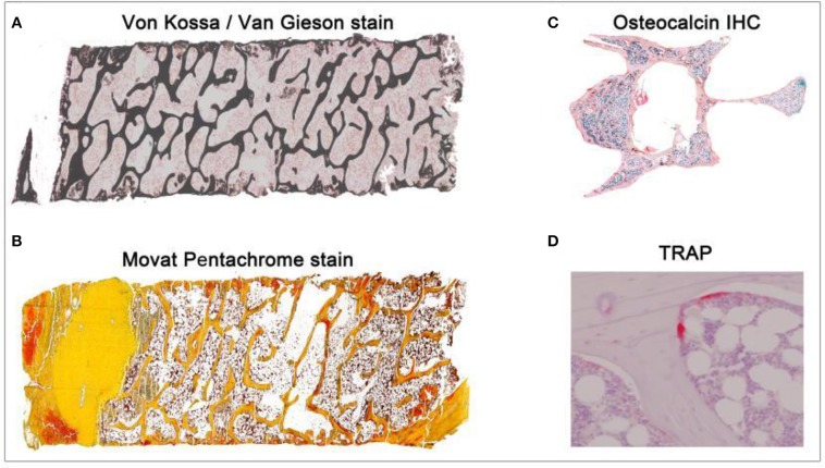
Figure 1
Overview of different histological stains evaluated using TWS and ImageJ toolbox. Sheep iliac crest biopsy and rat lumbar vertebral samples were used to test and set up the protocol. Sheep biopsy samp...
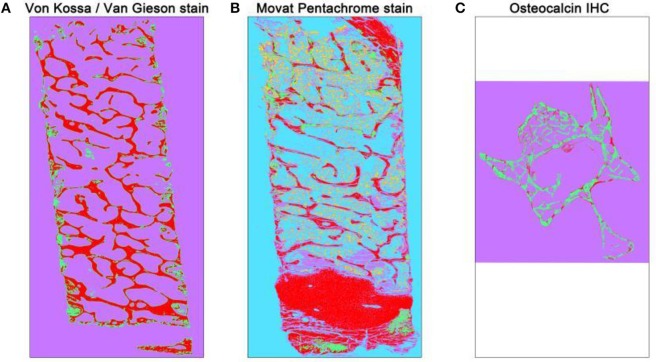
Figure 2
Overview of automated segmented images using TWS. The automated classification was carried out after training one stack of the whole overview image. Different histological stains were trained accordin...
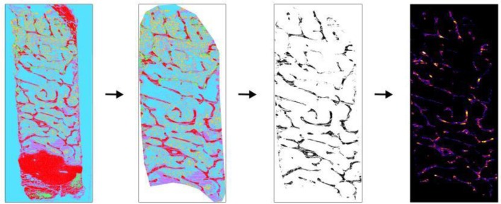
Figure 3
Application of BoneJ in the measurement of Tb.Th and Tb.Sp. Movat pentachrome stain classified overview of sheep iliac crest biopsy was used to obtain Tb.Th and Tb.Sp. (Left to right). The classified ...
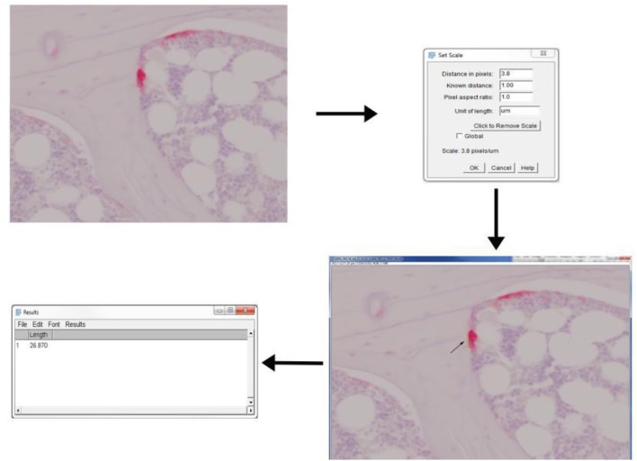
Figure 4
Application of ImageJ toolbox to measure osteoclast activity from TRAP stained sections. Rat vertebral sample was used to perform TRAP enzyme histochemistry. Osteoclasts are identified as multi-nuclea...
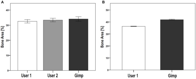
Figure 5
Comparison of TWS results analyzed by two different users and GIMP image analysis software. The reproducibility and validation of generated TWS script was tested by investigating inter-observer differ...
Figure images are served from the NIH/NLM PubMed Central Open Access Subset or Europe PMC; copyright remains with the publishers and authors.
💬 Discussion
0 commentsNo comments yet. Be the first to start a discussion!
Leave a Comment