Abstract
Abstract Pinpointing subcellular protein localizations from microscopy images is easy to the trained eye, but challenging to automate. Based on the Human Protein Atlas image collection, we held a competition to identify deep learning solutions to solve this task. Challenges included training on highly imbalanced classes and predicting multiple labels per image. Over 3 months, 2,172 teams participated. Despite convergence on popular networks and training techniques, there was considerable variety among the solutions. Participants applied strategies for modifying neural networks and loss functions, augmenting data and using pretrained networks. The winning models far outperformed our previous effort at multi-label classification of protein localization patterns by ~20%. These models can be used as classifiers to annotate new images, feature extractors to measure pattern similarity or pretrained networks for a wide range of biological applications.
🔬 Techniques
💻 Software
🧪 Sample Preparation
🔬 Cell Lines
🏭 Microscope Brands
💻 Software Details
📋 Protocols
💾 Data Repositories
🏛️ Research Organizations (ROR)
Affiliated research institutions:
📋 Methods
Competition and prizes This paper describes the outcome of the HPA Image Classification competition at Kaggle ( https://www.kaggle.com/c/human-protein-atlas-image-classification/ ), which was active from 3 October, 2018 to 10 January, 2019. The top-ranking solutions were awarded with a cash prize (Table 1 , first place, US$14,000; second place, US$10,000; third place, US$8,000 and fourth place, US$5,000).
Image generation in the HPA Cell Atlas
In the HPA Cell Atlas, each target protein is imaged in three different cell lines selected based on messenger RNA expression data from a large panel of cell lines. A standard immunostaining protocol is applied in a 96-well format to stain the target protein 49 ( https://www.protocols.io/view/standardized-immunohistochemical-staining-used-in-yj8furw ). To facilitate the downstream annotation process, reference markers for the nucleus, microtubules and endoplasmic reticulum are also stained. Confocal microscopes (63× oil immersion) are used to image each sample in the 96-well plate, and multiple images are typically acquired for each well. The four-color images (image size 2,048 × 2,048; 16-bit, pixel size 0.08 µm or 3,072 × 3,072; 16-bit, 0.08 µm) are uploaded to our laboratory information management system, where automatic quality checks are applied to pass only in-focus images with high contrast and good staining intensity. Manual annotation of the observed localization pattern is performed by applying one or more labels to the images (typically two to six) from each sample (same antibody, cell line and sample preparation date 3 ). This dataset contains a mixture of images annotated by two types of workflow: (1) experts annotate the image, another expert curates it and (2) gamers from EVE Online 5 annotate the images and the annotations are curated by experts, as described in (1). Typically, at least two images per antibody per cell line are selected to create the dataset. In HPAv18, 32 labels are used to describe cellular localization classes. Dataset assembly and quality control The total dataset consisted of 42,774 images. The training set had 31,072 images, and the test set had 11,702 images. We provided all images both in high resolution (a mix of 2,048 × 2,048 and 3,072 × 3,072 pixels, TIFF 8-bit image files) and low resolution (512 × 512 pixels, PNG 8-bit grayscale files). Note that the PNG files were directly resized from TIFF images. The size inconsistency for the TIFF images were due to the variation of the actual size of acquired area from the sample originally, but they all shared the same pixel resolution. A total of 32 organelle classes from the HPA were merged into 28 classes for the competition (see Supplementary Table 1 for details of how the classes were merged and Supplementary Table 2 for the distribution of the classes within the training and test sets). Since the HPA Cell Atlas includes over 30 different cell lines, we sampled across 27 main cell lines, and have a roughly equal distribution across different cell lines. Sampling was done in groups consisting of each cell line and organelle combination to achieve this effect. Still, some groups were smaller than others, due to the imbalanced nature of the total HPA data, both regarding the class labels applied and the cell lines used in the experiment (see Supplementary Table 3 for the cell type image distribution in the training and test sets). The test dataset images were collected first from nonpublished images generated within HPA. We excluded images from the same biological sample (with a specific protein and cell line) already represented in the test set from the training set to avoid information leakage. The training set images were collected from both public and nonpublic HPA Cell Atlas images. For quality control, we applied further image analysis to get an acceptable quality of the images in the competition dataset. This allowed us to use nonpublished images from the HPA Cell Atlas, which are of mixed quality (high and low) compared to the high quality of the published images. The quality control was based on cell count and image contrast. The cell count was performed on the red (microtubules) channel images, mainly by applying a Gaussian filter and otsu thresholding with the scikit-image 50 library and by removing objects smaller than 8,000 pixels. We required a minimum of five cells per image and excluded cells touching the image borders. A minimum contrast check was applied to the green channel (protein of interest) with the ‘is_low_contrast’ method from scikit-image. We set ‘fraction_threshold’ to 0.2 and ‘upper_percentile’ to 99.99. Low contrast images were discarded.
Show full methods section
Competition and prizes This paper describes the outcome of the HPA Image Classification competition at Kaggle ( https://www.kaggle.com/c/human-protein-atlas-image-classification/ ), which was active from 3 October, 2018 to 10 January, 2019. The top-ranking solutions were awarded with a cash prize (Table 1 , first place, US$14,000; second place, US$10,000; third place, US$8,000 and fourth place, US$5,000).
Image generation in the HPA Cell Atlas
In the HPA Cell Atlas, each target protein is imaged in three different cell lines selected based on messenger RNA expression data from a large panel of cell lines. A standard immunostaining protocol is applied in a 96-well format to stain the target protein 49 ( https://www.protocols.io/view/standardized-immunohistochemical-staining-used-in-yj8furw ). To facilitate the downstream annotation process, reference markers for the nucleus, microtubules and endoplasmic reticulum are also stained. Confocal microscopes (63× oil immersion) are used to image each sample in the 96-well plate, and multiple images are typically acquired for each well. The four-color images (image size 2,048 × 2,048; 16-bit, pixel size 0.08 µm or 3,072 × 3,072; 16-bit, 0.08 µm) are uploaded to our laboratory information management system, where automatic quality checks are applied to pass only in-focus images with high contrast and good staining intensity. Manual annotation of the observed localization pattern is performed by applying one or more labels to the images (typically two to six) from each sample (same antibody, cell line and sample preparation date 3 ). This dataset contains a mixture of images annotated by two types of workflow: (1) experts annotate the image, another expert curates it and (2) gamers from EVE Online 5 annotate the images and the annotations are curated by experts, as described in (1). Typically, at least two images per antibody per cell line are selected to create the dataset. In HPAv18, 32 labels are used to describe cellular localization classes. Dataset assembly and quality control The total dataset consisted of 42,774 images. The training set had 31,072 images, and the test set had 11,702 images. We provided all images both in high resolution (a mix of 2,048 × 2,048 and 3,072 × 3,072 pixels, TIFF 8-bit image files) and low resolution (512 × 512 pixels, PNG 8-bit grayscale files). Note that the PNG files were directly resized from TIFF images. The size inconsistency for the TIFF images were due to the variation of the actual size of acquired area from the sample originally, but they all shared the same pixel resolution. A total of 32 organelle classes from the HPA were merged into 28 classes for the competition (see Supplementary Table 1 for details of how the classes were merged and Supplementary Table 2 for the distribution of the classes within the training and test sets). Since the HPA Cell Atlas includes over 30 different cell lines, we sampled across 27 main cell lines, and have a roughly equal distribution across different cell lines. Sampling was done in groups consisting of each cell line and organelle combination to achieve this effect. Still, some groups were smaller than others, due to the imbalanced nature of the total HPA data, both regarding the class labels applied and the cell lines used in the experiment (see Supplementary Table 3 for the cell type image distribution in the training and test sets). The test dataset images were collected first from nonpublished images generated within HPA. We excluded images from the same biological sample (with a specific protein and cell line) already represented in the test set from the training set to avoid information leakage. The training set images were collected from both public and nonpublic HPA Cell Atlas images. For quality control, we applied further image analysis to get an acceptable quality of the images in the competition dataset. This allowed us to use nonpublished images from the HPA Cell Atlas, which are of mixed quality (high and low) compared to the high quality of the published images. The quality control was based on cell count and image contrast. The cell count was performed on the red (microtubules) channel images, mainly by applying a Gaussian filter and otsu thresholding with the scikit-image 50 library and by removing objects smaller than 8,000 pixels. We required a minimum of five cells per image and excluded cells touching the image borders. A minimum contrast check was applied to the green channel (protein of interest) with the ‘is_low_contrast’ method from scikit-image. We set ‘fraction_threshold’ to 0.2 and ‘upper_percentile’ to 99.99. Low contrast images were discarded.
Image-wise classification task
In this competition, the classification task is performed image-wise mostly because our current annotations are made at this level for each protein/antibody and cell line. We do not provide cell-wise labels, although it may yield better performance due to single-cell variations. However, we expect the impact to be minimal because only ~2% of proteins vary in their localization patterns between cells in images 3 and because these images are assigned the labels for all patterns observed in the image. Future improvements along this direction may be targeted to these proteins show single-cell variations.
Image resolutions and external data
We provide the entire image dataset in high and low resolutions, and we allowed the participants to explore the use of external data and pretrained models. We believe this is important, because it allowed the participants explore not only the model itself, but also different strategies to fetch external data, augment the data and take advantage of pretrained models, which had already been shown to be effective. We also believe it is important to obtain better performance under realistic constraints. For the hidden variable problem raised from the metric learning model, prohibiting the use of external training data (and pretrained networks) may reduce the same type of risk. However, this may also prevent teams from achieving the desired outcome, since external data can improve performance, as we observed with HPAv18. A compromise may be to restrict the set of information allowed for training, such as only location labels from HPAv18 to avoid finding weak correlations with extra information such as antibody identifiers.
Data leakage disclosure and fix during the competition
During the competition, participants notified us that there was a data leakage issue after comparing the public HPA Cell Atlas Images (HPAv18) with the test set images using similarity analysis (for example, perceptual image hashing). We identified that 148 out of 11,702 images in the test set (including ‘validation_public’ and ‘test_private’) were mistakenly included. We also noticed that all the leaked images contain rare class labels, and many of the leaked images were not identical to images in HPAv18 but highly similar, for example by coming from a different focal plane. Shortly after the leakage was identified, most of the leaked images in ‘test_private’ (the final evaluation test set to generate the ranking on the private leaderboard) were removed from scoring, and the rest of the leaked images were swapped with unleaked images with the same labels from ‘validation_public’ to keep rare classes in both test sets. All participants were notified of the leak and the fix. Most teams detected leaks in their code and excluded those leaked images from their own validation dataset. Performance criteria The F1 scores computed in Fig. 2 were computed from the following equation: documentclass[12pt]{minimal} usepackage{amsmath} usepackage{wasysym} usepackage{amsfonts} usepackage{amssymb} usepackage{amsbsy} usepackage{mathrsfs} usepackage{upgreek} setlength{oddsidemargin}{-69pt} begin{document}$${mathrm{Precision}} = frac{{T_{mathrm{p}}}}{{T_{mathrm{p}} + F_{mathrm{p}}}}$$end{document} Precision = T p T p + F p documentclass[12pt]{minimal} usepackage{amsmath} usepackage{wasysym} usepackage{amsfonts} usepackage{amssymb} usepackage{amsbsy} usepackage{mathrsfs} usepackage{upgreek} setlength{oddsidemargin}{-69pt} begin{document}$${mathrm{Recall}} = frac{{T_{mathrm{p}}}}{{T_{mathrm{p}} + F_{mathrm{n}}}}$$end{document} Recall = T p T p + F n documentclass[12pt]{minimal} usepackage{amsmath} usepackage{wasysym} usepackage{amsfonts} usepackage{amssymb} usepackage{amsbsy} usepackage{mathrsfs} usepackage{upgreek} setlength{oddsidemargin}{-69pt} begin{document}$${mathrm{F1}} = 2 times frac{{{mathrm{precision}} times {mathrm{recall}}}}{{{mathrm{precision}} + {mathrm{recall}}}}$$end{document} F1 = 2 × precision × recall precision + recall where T p denotes the number of images that are true positive, and F n , F p denote the false negative and false positive, respectively. The macro F1 score is computed from: documentclass[12pt]{minimal} usepackage{amsmath} usepackage{wasysym} usepackage{amsfonts} usepackage{amssymb} usepackage{amsbsy} usepackage{mathrsfs} usepackage{upgreek} setlength{oddsidemargin}{-69pt} begin{document}$${mathrm{macro}} {mathrm{F}}{1} = frac{1}{n}left( {mathop {sum }limits_{i = 1}^n {mathrm{F1}}} right)$$end{document} macro F 1 = 1 n ∑ i = 1 n F1 During the challenge, we used macro F1 to compute the score for public leaderboard rankings. Each team was allowed to select two final submissions at the end of the challenge. Macro F1 was used to compute the score on the private leaderboard (if there were two submissions for a team, we took the maximum score), and this was used as the main criterion to award the teams. To analyze the score distributions of all teams, we took the one submission per team that gave the maximum score on the private leaderboard. For Fig. 2d we computed the score for all, single- and multi-localized classes with macro F1. Per-class F1 scores in Fig. 2c were computed with F1 for each class with no averaging. Scores shown in tables were rounded down. Public and private leaderboard During the competition, teams were scored and ranked on a public leaderboard. To prevent overfitting to the public leaderboard, a subset (29%) of the test set was used for calculating the leaderboard scores, while the remaining part (71%) of the test set was preserved for the final evaluation. This is important because participants tend to optimize toward higher scores on the public leaderboard at the risk of overfitting to the test data. Since the participants ran their own model and only submitted the predicted labels for the test set, it was mandatory for the top four winning teams to submit their models for further inspection. CAMs We used Grad-CAM 40 to produce the CAMs shown in Fig. 3 and Supplementary Fig. 13 from a chosen reference convolutional layer of the network under investigation. We generated CAMs for the following models in Fig. 3 : Model 1 is densenet121_1024 from Team 1, Model 2 is inception-v3 from Team 3, Model 3 is densenet121_standard_no_crop and the metric learning model from Team 1. The architecture of these three models are shown in Supplementary Fig. 12 . For generating CAMs, the reference convolutional layer of these models was set to Block3, Mixed_7c, Layer3 and Layer3, respectively. The generated CAMs were resized and overlaid on top of the corresponding input image. These models are also described in Supplementary Notes : experiment 18 in Supplementary Table 5b , experiment 8 in Supplementary Table 5f , experiment 30 in Supplementary Table 5b and model 5 in Supplementary Table 5a . Feature visualization with UMAP For the feature visualization in Fig. 4 , we used the 1,024-dimension feature from the ‘fc’ layer (as shown in Supplementary Fig. 12 ) of the densenet121_1024 model from Team 1. It was projected with UMAP to reduce the dimensionality from 1024 to 2. For generating the UMAP, the number of neighboring points, minimal point distance and number of components metric were set to 15, 0.1 and 2, respectively. The distance metric was set to Euclidean distance. We processed all the images in the training set and the entire HPAv18 dataset, and the generated 2D vectors were then plotted as a scatter plot. The data points are color coded are corresponding to their annotated location. For the live HPA-UMAP ( https://tinyurl.com/y6nhf5bo ), we wrote the ImJoy plugin in Javascript and used Plotly.js to make the plot. Images shown when clicking the data points were pulled from the proteinatlas.org dynamically.
Metric learning model results evaluation
The score boost for the metric learning is mostly because of identification of ‘batch effects’ defined as images derived from different regions of the exact same sample (antibody and cell line combination), and not mainly from improved performance for rare classes. In total, 935 images in the ‘test_private’ set has one other image from the same sample in HPAv18 and the metric learning model detects 647 (69.2%) of them. We found 270 images in the ‘test_private’ set where the classification model made wrong predictions, but were successfully corrected by the metric learning model. Among these images, 261 have at least one image from the same sample in HPAv18 and 34 of them belong to rare classes (rare class defined as containing fewer than 1,000 images in the dataset). However, there are 71 images from the ‘test_private’ set (including five rare images) that were correctly predicted by the classification model, but replaced into wrong labels by the metric learning model.
Statistical analysis
The plotting and statistical analysis were performed with Python 3.6, NumPy, SciPy, scikit-learn, Pandas, seaborn and Matplotlib. To test the Macro F1 score difference between single label and multi-label images a two-sample Kolmogorov–Smirnov test was performed for significance testing. The test returns a two-tailed P value. The scores for single label images are significantly higher ( P < 1.08 × 10 −5 ) than for multi-label images for all groups. The test was done for each group of teams, 1–10: n = 10 teams ( P < 1.08 × 10 −5 ), 11–100: n = 90 teams ( P < 3.96 × 10 −51 ), 101–500: n = 400 teams ( P < 5.22 × 10 −197 ) and 501–2,137: n = 1,637 teams ( P < 4.01 × 10 −186 ). Reporting Summary Further information on research design is available in the Nature Research Reporting Summary linked to this article.
Online content Any methods, additional references, Nature Research reporting summaries, source data, extended data, supplementary information, acknowledgements, peer review information, details of author contributions and competing interests, and statements of code and data availability are available at 10.1038/s41592-019-0658-6.
Supplementary information Supplementary Information Supplementary Figs. 1–13, Tables 1–9 and Notes 1–9. Reporting Summary Supplementary Table 4 Class-wise score for the nine invited teams, Macro F1 score per class for each of the invited teams in the competition. Supplementary Table 5 Models and ablation study from the nine selected teams, Description of the different models used by the invited teams as well as an analysis of what factors contributed the most to the performance of the models.
📊 Figures
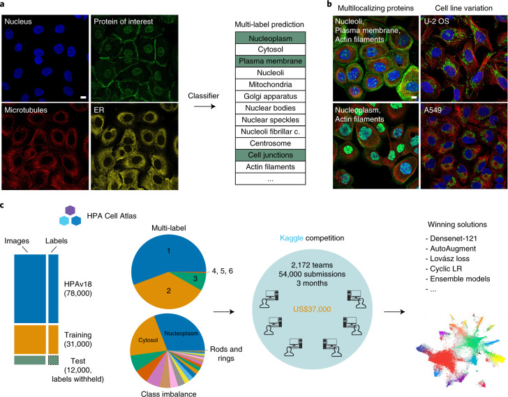
Fig. 1
Overview of image dataset and challenge design.
a , A typical HPA Cell Atlas image and the aim of the competition. Each image consists of four channels: the antibody-stained protein of interest (green) and three reference channels to outline the ce...
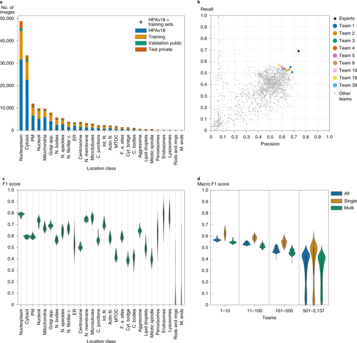
Fig. 2
Competition results.
a , Image numbers of each localization class for HPAv18, training, validation_public and test_private dataset. PM, plasma membrane; Golgi app., Golgi apparatus; N. bodies, nuclear bodies; N. speckles,...
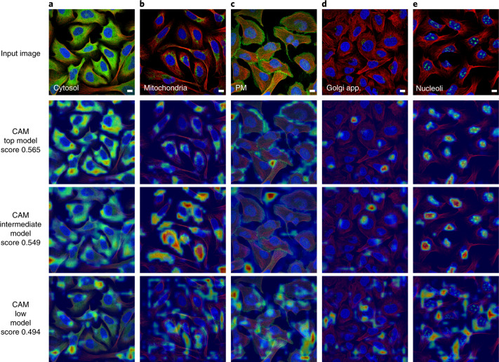
Fig. 3
Visualization of model spatial attention.
CAMs for three different models, the top-scoring model (from Team 1), an intermediate-scoring model (from Team 3) and a low-scoring model (from Team 1). Scale bars, 10u2009u03bcm. a , For the cytosoli...
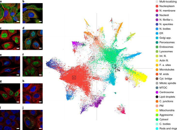
Fig. 4
Visualization of learned features.
UMAP visualization of the features learned by the best scoring model from Team 1 with a few corresponding original images highlighted. Single location images are colored according to location, while g...
Figure images are served from the NIH/NLM PubMed Central Open Access Subset or Europe PMC; copyright remains with the publishers and authors.
💬 Discussion
0 commentsNo comments yet. Be the first to start a discussion!
Leave a Comment