Abstract
AbstractPorosity and permeability are the key factors in assessing the hydrocarbon productivity of unconventional (shale) reservoirs, which are complex in nature due to their heterogeneous mineralogy and poorly connected nano- and micro-pore systems. Experimental efforts to measure these petrophysical properties posse many limitations, because they often take weeks to complete and are difficult to reproduce. Alternatively, numerical simulations can be conducted in digital rock 3D models reconstructed from image datasets acquired via e.g., nanoscale-resolution focused ion beam–scanning electron microscopy (FIB-SEM) nano-tomography. In this study, impact of reservoir confinement (stress) on porosity and permeability of shales was investigated using two digital rock 3D models, which represented nanoporous organic/mineral microstructure of the Marcellus Shale. Five stress scenarios were simulated for different depths (2,000–6,000 feet) within the production interval of a typical oil/gas reservoir within the Marcellus Shale play. Porosity and permeability of the pre- and post-compression digital rock 3D models were calculated and compared. A minimal effect of stress on porosity and permeability was observed in both 3D models. These results have direct implications in determining the oil-/gas-in-place and assessing the production potential of a shale reservoir under various stress conditions.
🔬 Techniques
💻 Software
🏭 Microscope Brands
🧪 Reagent Suppliers
💻 Software Details
🏛️ Research Organizations (ROR)
Affiliated research institutions:
📋 Methods
Traditional core analytical techniques commonly used to determine porosity or permeability of oil-/gas-bearing rocks, developed for conventional (sandstone or carbonate) reservoirs, are limited in terms of characterizing unconventional (shale) reservoirs. This adds to the difficulties of exploration intended for production which requires a search for a new solution to supplement the existing characterization methods. Petroleum industry is now turning to the technique of “digital rock” as a potential solution for characterizing shales, owing to the power of modern microscopes to reliably and precisely image and analyze these rocks at the micro- and/or nanoscale-resolution. Digital rock analysis (also known as digital rock physics) integrates multi-scale and multi-modal 2D/3D imaging techniques (e.g., field-emission scanning electron microscopy (FE-SEM) or focused ion beam – scanning electron microscopy (FIB-SEM) nano-tomography) together with advanced image analysis methods. These digital rock 3D models can be then used to investigate e.g., nanoporous microstructure of geomaterials in very fine detail, or for modeling and simulation of various multi-physics processes that take place within these geosystems deep in the subsurface.
Nanoscale-resolution 3D imaging with focused ion beam–scanning electron microscopy
(FIB-SEM) nano-tomography FIB-SEM nano-tomography (serial-sectioning) is a nanoscale-resolution 3D imaging technique in which cross-section ion milling is used to controllably remove approximately 5- to 20-nm-thin layer of material (“slice”) of the sample, and electron imaging is used to characterize the freshly prepared sample surface. Automated sequential FIB milling and SEM imaging allows for the acquisition of a series of images, which in turn leads to digital rock 3D model reconstruction. In this study, a ZEISS Crossbeam 550 FIB-SEM was used to collect ultra-high-resolution (5 nm/voxel) image datasets of two organic-rich regions of interest (ROIs) of a Marcellus Shale rock sample. Both, secondary electron (SE) and backscatter electron (BSE) signals were acquired at the time of the 3D imaging. These SE and BSE images were then blended into a single image dataset to optimize brightness and contrast between organic, mineral, and pore phases. Image analysis: image processing and (machine learning) image segmentation Image processing was first performed in order to improve image quality – a combination of different filters and operations was applied in order to remove imaging artifacts, noise, and other background intensity variations from the images. Commonly found artifacts in FIB-SEM nano-tomography image datasets are e.g., curtaining or shadowing effect. These can be removed by applying various image processing algorithms (e.g., FFT, local or non-local means filters). Image segmentation, on the other hand, allows for classification of the images into segments representing different (shale rock) material components (of different densities, and hence of different intensities in the images). In this study, machine learning segmentation was applied in order to segment pore, organic, and non-organic (mineral) phases within the FIB-SEM nano-tomography image datasets. In the past decade, machine learning grew out of the quest for artificial intelligence and has found application in many areas (e.g., self-driving cars, effective web search), however its application to image analysis has been recently developed. Machine learning algorithms enable it to identify patterns in observed data and build predictive models without being explicitly programmed. Machine learning image segmentation automatically partition challenging image datasets, that may carry a variety of modality-specific imaging artifacts, into segments (labels), representing different groups of features of the rock microstructure (e.g., pores or minerals), previously too difficult to segment by threshold- or watershed-based approaches 39 . Machine learning image segmentation was performed with the ZEN Intellesis software, developed by ZEISS, which uses open-source packages (such as scikit-image and SciPy) for feature extraction. The machine learning capability allows for interactive training of the microscopy 2D/3D images. A combination of different filters (e.g., mean, Gaussian, Gabor, Hessian, Sobel) are used to extract relevant features from each greyscale channel of an image. A machine learning algorithm – forest of randomized trees – is used to train the segmentation model (classifier). The classifier is then applied to a slice displayed or a 3D volume. This process is iterative where additional data may be added to refine the segmentation of a 2D slice or a 3D volume. The final segmented 2D/3D image is produced by using the satisfactorily-trained segmentation model to the entire image dataset 40 . The processed and segmented image datasets were then reconstructed into two digital rock 3D models: ROI-1 (3.25 µm × 2.5 µm × 2.5 µm) and ROI-2 (3.75 µm × 2.25 µm × 2 µm). These two 3D models were then used for mechanics (compression) and fluid flow (permeability) simulations performed using the GeoDict software. The GeoDict software, developed by Math2Market, brings different solution methods into play for the simulation of mechanics and single-phase flow in porous media 41 . The common denominator of the computational models (solvers), used in this software, is that they work directly on 3D models. They do not require a mesh generation step, which is a bottleneck for classical finite-element or finite-volume methods. Mechanics (compression) simulations For a uniform macroscopic strain S , the boundary value problem (BVP) for the stress field σ , strain field ε , and displacement field μ * can be stated. The BVP or equations of linear elasticity consists of the elastic equilibrium Eq. ( 1 ), Hooke’s law (2), and periodic boundary conditions (3): 1 documentclass[12pt]{minimal} usepackage{amsmath} usepackage{wasysym} usepackage{amsfonts} usepackage{amssymb} usepackage{amsbsy} usepackage{mathrsfs} usepackage{upgreek} setlength{oddsidemargin}{-69pt} begin{document}$$nabla cdot sigma =0$$end{document} ∇ ⋅ σ = 0 2 documentclass[12pt]{minimal} usepackage{amsmath} usepackage{wasysym} usepackage{amsfonts} usepackage{amssymb} usepackage{amsbsy} usepackage{mathrsfs} usepackage{upgreek} setlength{oddsidemargin}{-69pt} begin{document}$$sigma =C:{epsilon }$$end{document} σ = C : ϵ 3 documentclass[12pt]{minimal} usepackage{amsmath} usepackage{wasysym} usepackage{amsfonts} usepackage{amssymb} usepackage{amsbsy} usepackage{mathrsfs} usepackage{upgreek} setlength{oddsidemargin}{-69pt} begin{document}$$2{epsilon }=2S+nabla {u}^{ast }+{(nabla {u}^{ast })}^{T}$$end{document} 2 ϵ = 2 S + ∇ u ∗ + ( ∇ u ∗ ) T By introducing a reference material of homogeneous stiffness C 0 ., the BVP can be transformed into the strain-based Lippmann-Schwinger Eq. ( 4 ): 4 documentclass[12pt]{minimal} usepackage{amsmath} usepackage{wasysym} usepackage{amsfonts} usepackage{amssymb} usepackage{amsbsy} usepackage{mathrsfs} usepackage{upgreek} setlength{oddsidemargin}{-69pt} begin{document}$$(I+{B}_{{epsilon }}){epsilon }=epsilon +{Gamma }_{0}ast ((C-{C}_{0}):{epsilon })=E$$end{document} ( I + B ϵ ) ϵ = ϵ + Γ 0 ∗ ( ( C − C 0 ) : ϵ ) = E Fast Fourier transform (FFT) allows to solve the convolution wh the Green’s operator Γ 0 42 . The Lippmann-Schwinger equation can also bformulated with respect of stress instead of strain. These equations can iteratively be solved using the Neumann series expansion, the so-called “basis scheme”. Instead of using the Nmann series expansion, Krylov subspace methods can be applied to accelerate the convergence of the method. The formulation allows to handle linear and non-linear (i.e., replacing Hooke’s law with a non-linear formulation) material laws as well as isotropic, transverse-isotropic, orthotropic, or anisotropic constituent materials. Similar to the fluid flow solvers (described below), a staggered grid is used to discretize displacement, strain, and stress variables 43 . For the computation of compression dependent properties, the displacement field μ *. used to predict a compressed structure. The voxels of the original image are moved along the displacement field and cut with a reduced voxel image. The result of that procedure is a grayscale image, where a global threshold is used to perform a segmentation of the different phases. The threshold is chosen in the FeelMath solver such that either mass or volume is preserved. Fluid flow (permeability) simulations A laminar flow of aluid with constant viscosity μ , velocity μ , and pressure p are described by Stokes conservation of momentum (5), conservation of mass (6), and no-slip boundary conditions (7). The domain Ω is periodic and the direction of the flow is induced by the unit vector f . that always points in the direction of one of the coordinate axes: 5 documentclass[12pt]{minimal} usepackage{amsmath} usepackage{wasysym} usepackage{amsfonts} usepackage{amssymb} usepackage{amsbsy} usepackage{mathrsfs} usepackage{upgreek} setlength{oddsidemargin}{-69pt} begin{document}$${rm{mu }}{nabla }^{2}{rm{u}}-nabla {rm{p}}={f}$$end{document} μ ∇ 2 u − ∇ p = f 6 documentclass[12pt]{minimal} usepackage{amsmath} usepackage{wasysym} usepackage{amsfonts} usepackage{amssymb} usepackage{amsbsy} usepackage{mathrsfs} usepackage{upgreek} setlength{oddsidemargin}{-69pt} begin{document}$$nabla cdot u=0$$end{document} ∇ ⋅ u = 0 7 documentclass[12pt]{minimal} usepackage{amsmath} usepackage{wasysym} usepackage{amsfonts} usepackage{amssymb} usepackage{amsbsy} usepackage{mathrsfs} usepackage{upgreek} setlength{oddsidemargin}{-69pt} begin{document}$$u{|}_{partial Omega }=0$$end{document} u | ∂ Ω = 0 The no-slip boundary conditions (7) are applicable forlow movement of fluid in the porous media. Following the set of Eqs. ( 5 , 6 , and 7 ), a few fluid flow simulations are conducted in the digital rock 3D models to calculate effective material properties, such as permeability. In these simulations, the mean flow velocity is measured for an applied pressure drop across the porous media. Although the Eqs. 5 , 6 , and 7 ) do not contain permeability ( K ) term, it is calculated during post-processing step. The relationship between the predicted mean flow velocity for a pressure drop in a porous media is expressed by a constitutive equation, commonly-known as Darcy’s law ( 8 ): 8 documentclass[12pt]{minimal} usepackage{amsmath} usepackage{wasysym} usepackage{amsfonts} usepackage{amssymb} usepackage{amsbsy} usepackage{mathrsfs} usepackage{upgreek} setlength{oddsidemargin}{-69pt} begin{document}$$u=-,frac{K}{{rm{mu }}}(nabla {rm{p}}-f)$$end{document} u = − K μ ( ∇ p − f ) where K is the permeability of the material. In the Stokes flow regime, average velocity changes linearly with pressure drop, as shown in Fig. 10 as an example. The slope of this straight line is essentially the ratio of permeability of material and viscosity of fluid according to Darcy’s law (8). Figure 10 A linear relationship between pressure drop and average flow velocity in porous media. The left identity right (LIR) solver 44 (a fast and memory-efficient iterative finite volume method) was used for fluid flow simulations. The solver computes the permeability, as well as velocity and pressure fields, on 3D models. The LIR solver can be used for the numerical solution of the Stokes, Stokes-Brinkman, Navier-Stokes, and Navier-Stokes-Brinkman equations. Usually, 3D models are represented as regular voxel grids where the number of grid cells grows cubically. The LIR solver uses an adaptive grid, instead of a regular grid, to reduce the number of grid cells significantly. The basis of the adaptive grid is a data structure called LIR-tree 45 that is used for spatial partitioning of 3D models. The pore space is coarsened in areas with small velocity and pressure variations, while keeping the original resolution near the solid surfaces and in regions where velocity or pressure vary rapidly. Pressure and velocity are discretized on staggered grids and they are arranged in such a way that each cell can satisfy the (Navier-)Stokes(-Brinkman) equations independently from its neighbor cells. Pressure variables represent an average for the whole cube and residue at the cube centers, whereas the velocities represent transport across faces between the cubes and residue on the respective faces of the cube. Two velocity variables, namely one for each neighboring cell, are introduced instead of using one velocity variable on the cell faces. The two velocity variables discretize the two one-sided limits at the center of the cell surface. The discretization of the momentum and mass conservation equations yields one linear system (block) per cell. This block structure allows using the block Gauß-Seidel algorithm as smoother in a multigrid approach as an iterative solver method.
Show full methods section
Traditional core analytical techniques commonly used to determine porosity or permeability of oil-/gas-bearing rocks, developed for conventional (sandstone or carbonate) reservoirs, are limited in terms of characterizing unconventional (shale) reservoirs. This adds to the difficulties of exploration intended for production which requires a search for a new solution to supplement the existing characterization methods. Petroleum industry is now turning to the technique of “digital rock” as a potential solution for characterizing shales, owing to the power of modern microscopes to reliably and precisely image and analyze these rocks at the micro- and/or nanoscale-resolution. Digital rock analysis (also known as digital rock physics) integrates multi-scale and multi-modal 2D/3D imaging techniques (e.g., field-emission scanning electron microscopy (FE-SEM) or focused ion beam – scanning electron microscopy (FIB-SEM) nano-tomography) together with advanced image analysis methods. These digital rock 3D models can be then used to investigate e.g., nanoporous microstructure of geomaterials in very fine detail, or for modeling and simulation of various multi-physics processes that take place within these geosystems deep in the subsurface.
Nanoscale-resolution 3D imaging with focused ion beam–scanning electron microscopy
(FIB-SEM) nano-tomography FIB-SEM nano-tomography (serial-sectioning) is a nanoscale-resolution 3D imaging technique in which cross-section ion milling is used to controllably remove approximately 5- to 20-nm-thin layer of material (“slice”) of the sample, and electron imaging is used to characterize the freshly prepared sample surface. Automated sequential FIB milling and SEM imaging allows for the acquisition of a series of images, which in turn leads to digital rock 3D model reconstruction. In this study, a ZEISS Crossbeam 550 FIB-SEM was used to collect ultra-high-resolution (5 nm/voxel) image datasets of two organic-rich regions of interest (ROIs) of a Marcellus Shale rock sample. Both, secondary electron (SE) and backscatter electron (BSE) signals were acquired at the time of the 3D imaging. These SE and BSE images were then blended into a single image dataset to optimize brightness and contrast between organic, mineral, and pore phases. Image analysis: image processing and (machine learning) image segmentation Image processing was first performed in order to improve image quality – a combination of different filters and operations was applied in order to remove imaging artifacts, noise, and other background intensity variations from the images. Commonly found artifacts in FIB-SEM nano-tomography image datasets are e.g., curtaining or shadowing effect. These can be removed by applying various image processing algorithms (e.g., FFT, local or non-local means filters). Image segmentation, on the other hand, allows for classification of the images into segments representing different (shale rock) material components (of different densities, and hence of different intensities in the images). In this study, machine learning segmentation was applied in order to segment pore, organic, and non-organic (mineral) phases within the FIB-SEM nano-tomography image datasets. In the past decade, machine learning grew out of the quest for artificial intelligence and has found application in many areas (e.g., self-driving cars, effective web search), however its application to image analysis has been recently developed. Machine learning algorithms enable it to identify patterns in observed data and build predictive models without being explicitly programmed. Machine learning image segmentation automatically partition challenging image datasets, that may carry a variety of modality-specific imaging artifacts, into segments (labels), representing different groups of features of the rock microstructure (e.g., pores or minerals), previously too difficult to segment by threshold- or watershed-based approaches 39 . Machine learning image segmentation was performed with the ZEN Intellesis software, developed by ZEISS, which uses open-source packages (such as scikit-image and SciPy) for feature extraction. The machine learning capability allows for interactive training of the microscopy 2D/3D images. A combination of different filters (e.g., mean, Gaussian, Gabor, Hessian, Sobel) are used to extract relevant features from each greyscale channel of an image. A machine learning algorithm – forest of randomized trees – is used to train the segmentation model (classifier). The classifier is then applied to a slice displayed or a 3D volume. This process is iterative where additional data may be added to refine the segmentation of a 2D slice or a 3D volume. The final segmented 2D/3D image is produced by using the satisfactorily-trained segmentation model to the entire image dataset 40 . The processed and segmented image datasets were then reconstructed into two digital rock 3D models: ROI-1 (3.25 µm × 2.5 µm × 2.5 µm) and ROI-2 (3.75 µm × 2.25 µm × 2 µm). These two 3D models were then used for mechanics (compression) and fluid flow (permeability) simulations performed using the GeoDict software. The GeoDict software, developed by Math2Market, brings different solution methods into play for the simulation of mechanics and single-phase flow in porous media 41 . The common denominator of the computational models (solvers), used in this software, is that they work directly on 3D models. They do not require a mesh generation step, which is a bottleneck for classical finite-element or finite-volume methods. Mechanics (compression) simulations For a uniform macroscopic strain S , the boundary value problem (BVP) for the stress field σ , strain field ε , and displacement field μ * can be stated. The BVP or equations of linear elasticity consists of the elastic equilibrium Eq. ( 1 ), Hooke’s law (2), and periodic boundary conditions (3): 1 documentclass[12pt]{minimal} usepackage{amsmath} usepackage{wasysym} usepackage{amsfonts} usepackage{amssymb} usepackage{amsbsy} usepackage{mathrsfs} usepackage{upgreek} setlength{oddsidemargin}{-69pt} begin{document}$$nabla cdot sigma =0$$end{document} ∇ ⋅ σ = 0 2 documentclass[12pt]{minimal} usepackage{amsmath} usepackage{wasysym} usepackage{amsfonts} usepackage{amssymb} usepackage{amsbsy} usepackage{mathrsfs} usepackage{upgreek} setlength{oddsidemargin}{-69pt} begin{document}$$sigma =C:{epsilon }$$end{document} σ = C : ϵ 3 documentclass[12pt]{minimal} usepackage{amsmath} usepackage{wasysym} usepackage{amsfonts} usepackage{amssymb} usepackage{amsbsy} usepackage{mathrsfs} usepackage{upgreek} setlength{oddsidemargin}{-69pt} begin{document}$$2{epsilon }=2S+nabla {u}^{ast }+{(nabla {u}^{ast })}^{T}$$end{document} 2 ϵ = 2 S + ∇ u ∗ + ( ∇ u ∗ ) T By introducing a reference material of homogeneous stiffness C 0 ., the BVP can be transformed into the strain-based Lippmann-Schwinger Eq. ( 4 ): 4 documentclass[12pt]{minimal} usepackage{amsmath} usepackage{wasysym} usepackage{amsfonts} usepackage{amssymb} usepackage{amsbsy} usepackage{mathrsfs} usepackage{upgreek} setlength{oddsidemargin}{-69pt} begin{document}$$(I+{B}_{{epsilon }}){epsilon }=epsilon +{Gamma }_{0}ast ((C-{C}_{0}):{epsilon })=E$$end{document} ( I + B ϵ ) ϵ = ϵ + Γ 0 ∗ ( ( C − C 0 ) : ϵ ) = E Fast Fourier transform (FFT) allows to solve the convolution wh the Green’s operator Γ 0 42 . The Lippmann-Schwinger equation can also bformulated with respect of stress instead of strain. These equations can iteratively be solved using the Neumann series expansion, the so-called “basis scheme”. Instead of using the Nmann series expansion, Krylov subspace methods can be applied to accelerate the convergence of the method. The formulation allows to handle linear and non-linear (i.e., replacing Hooke’s law with a non-linear formulation) material laws as well as isotropic, transverse-isotropic, orthotropic, or anisotropic constituent materials. Similar to the fluid flow solvers (described below), a staggered grid is used to discretize displacement, strain, and stress variables 43 . For the computation of compression dependent properties, the displacement field μ *. used to predict a compressed structure. The voxels of the original image are moved along the displacement field and cut with a reduced voxel image. The result of that procedure is a grayscale image, where a global threshold is used to perform a segmentation of the different phases. The threshold is chosen in the FeelMath solver such that either mass or volume is preserved. Fluid flow (permeability) simulations A laminar flow of aluid with constant viscosity μ , velocity μ , and pressure p are described by Stokes conservation of momentum (5), conservation of mass (6), and no-slip boundary conditions (7). The domain Ω is periodic and the direction of the flow is induced by the unit vector f . that always points in the direction of one of the coordinate axes: 5 documentclass[12pt]{minimal} usepackage{amsmath} usepackage{wasysym} usepackage{amsfonts} usepackage{amssymb} usepackage{amsbsy} usepackage{mathrsfs} usepackage{upgreek} setlength{oddsidemargin}{-69pt} begin{document}$${rm{mu }}{nabla }^{2}{rm{u}}-nabla {rm{p}}={f}$$end{document} μ ∇ 2 u − ∇ p = f 6 documentclass[12pt]{minimal} usepackage{amsmath} usepackage{wasysym} usepackage{amsfonts} usepackage{amssymb} usepackage{amsbsy} usepackage{mathrsfs} usepackage{upgreek} setlength{oddsidemargin}{-69pt} begin{document}$$nabla cdot u=0$$end{document} ∇ ⋅ u = 0 7 documentclass[12pt]{minimal} usepackage{amsmath} usepackage{wasysym} usepackage{amsfonts} usepackage{amssymb} usepackage{amsbsy} usepackage{mathrsfs} usepackage{upgreek} setlength{oddsidemargin}{-69pt} begin{document}$$u{|}_{partial Omega }=0$$end{document} u | ∂ Ω = 0 The no-slip boundary conditions (7) are applicable forlow movement of fluid in the porous media. Following the set of Eqs. ( 5 , 6 , and 7 ), a few fluid flow simulations are conducted in the digital rock 3D models to calculate effective material properties, such as permeability. In these simulations, the mean flow velocity is measured for an applied pressure drop across the porous media. Although the Eqs. 5 , 6 , and 7 ) do not contain permeability ( K ) term, it is calculated during post-processing step. The relationship between the predicted mean flow velocity for a pressure drop in a porous media is expressed by a constitutive equation, commonly-known as Darcy’s law ( 8 ): 8 documentclass[12pt]{minimal} usepackage{amsmath} usepackage{wasysym} usepackage{amsfonts} usepackage{amssymb} usepackage{amsbsy} usepackage{mathrsfs} usepackage{upgreek} setlength{oddsidemargin}{-69pt} begin{document}$$u=-,frac{K}{{rm{mu }}}(nabla {rm{p}}-f)$$end{document} u = − K μ ( ∇ p − f ) where K is the permeability of the material. In the Stokes flow regime, average velocity changes linearly with pressure drop, as shown in Fig. 10 as an example. The slope of this straight line is essentially the ratio of permeability of material and viscosity of fluid according to Darcy’s law (8). Figure 10 A linear relationship between pressure drop and average flow velocity in porous media. The left identity right (LIR) solver 44 (a fast and memory-efficient iterative finite volume method) was used for fluid flow simulations. The solver computes the permeability, as well as velocity and pressure fields, on 3D models. The LIR solver can be used for the numerical solution of the Stokes, Stokes-Brinkman, Navier-Stokes, and Navier-Stokes-Brinkman equations. Usually, 3D models are represented as regular voxel grids where the number of grid cells grows cubically. The LIR solver uses an adaptive grid, instead of a regular grid, to reduce the number of grid cells significantly. The basis of the adaptive grid is a data structure called LIR-tree 45 that is used for spatial partitioning of 3D models. The pore space is coarsened in areas with small velocity and pressure variations, while keeping the original resolution near the solid surfaces and in regions where velocity or pressure vary rapidly. Pressure and velocity are discretized on staggered grids and they are arranged in such a way that each cell can satisfy the (Navier-)Stokes(-Brinkman) equations independently from its neighbor cells. Pressure variables represent an average for the whole cube and residue at the cube centers, whereas the velocities represent transport across faces between the cubes and residue on the respective faces of the cube. Two velocity variables, namely one for each neighboring cell, are introduced instead of using one velocity variable on the cell faces. The two velocity variables discretize the two one-sided limits at the center of the cell surface. The discretization of the momentum and mass conservation equations yields one linear system (block) per cell. This block structure allows using the block Gauß-Seidel algorithm as smoother in a multigrid approach as an iterative solver method.
📊 Figures
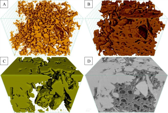
Figure 1
Visualization of segmented ( A ) pores, ( B ) organic matter, and ( C ) mineral phases present within digital rock 3D model reconstructed from ( D ) FIB-SEM nano-tomography image dataset of the ROI-1.
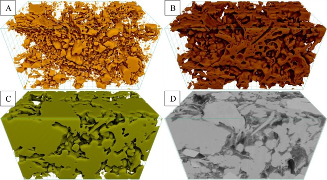
Figure 2
Visualization of segmented ( A ) pores, ( B ) organic matter, and ( C ) mineral phases present within digital rock 3D model reconstructed from ( D ) FIB-SEM nano-tomography image dataset of the ROI-2.
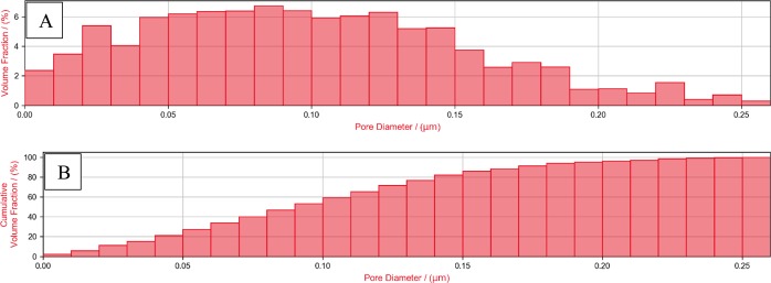
Figure 3
( A ) Relative and ( B ) cumulative pore size distribution (PSD) of the ROI-1 3D model.
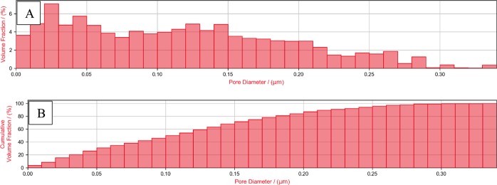
Figure 4
( A ) Relative and ( B ) cumulative pore size distribution (PSD) of the ROI-2 3D model.
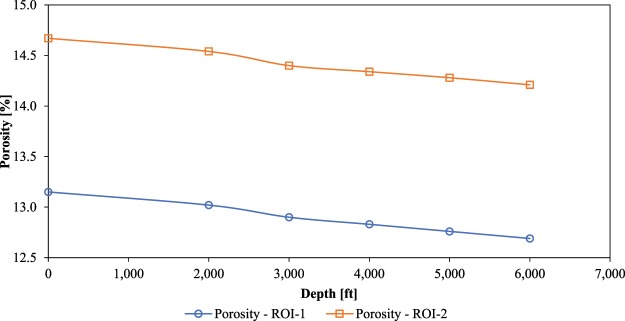
Figure 5
Porosity of the ROI-1 and ROI-2 3D models after five compression simulations.
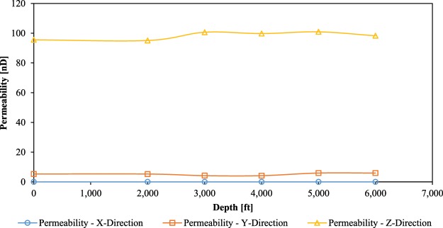
Figure 6
Permeabilities of the ROI-1 3D model after five compression simulations.
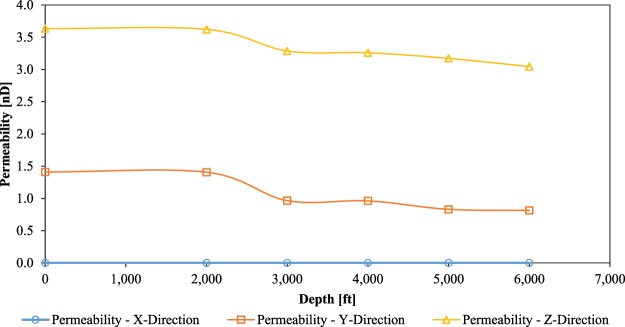
Figure 7
Permeabilities of the ROI-2 3D model after five compression simulations.
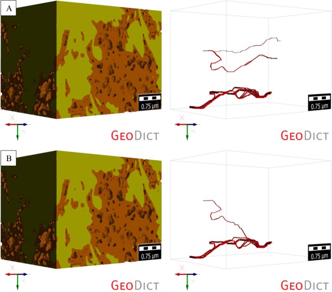
Figure 8
Visualization of the percolation paths of the ( A ) non-compressed and ( B ) compressed (at the maximum depth of 6,000u2009ft) ROI-1.
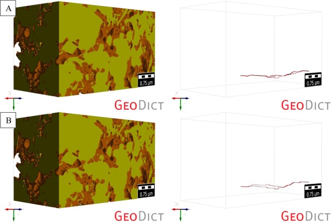
Figure 9
Visualization of the percolation paths of the ( A ) non-compressed and ( B ) compressed (at the maximum depth of 6,000u2009ft) ROI-2.
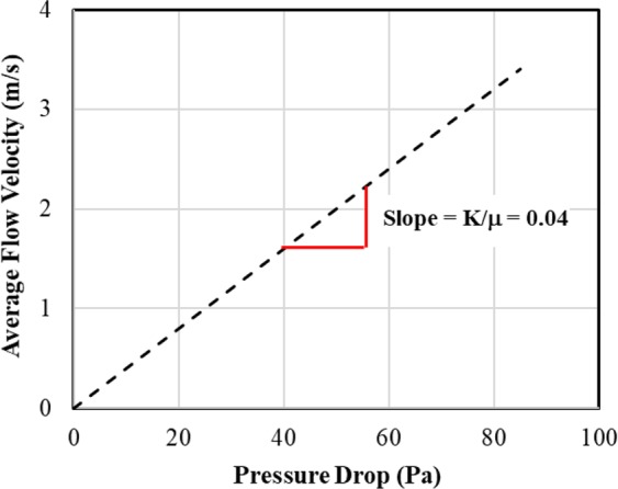
Figure 10
A linear relationship between pressure drop and average flow velocity in porous media.
Figure images are served from the NIH/NLM PubMed Central Open Access Subset or Europe PMC; copyright remains with the publishers and authors.
💬 Discussion
0 commentsNo comments yet. Be the first to start a discussion!
Leave a Comment