Abstract
The proteasome is an ATP-dependent, 2.5-megadalton molecular machine that is responsible for selective protein degradation in eukaryotic cells. Here we present cryo-electron microscopy structures of the substrate-engaged human proteasome in seven conformational states at 2.8-3.6 Å resolution, captured during breakdown of a polyubiquitylated protein. These structures illuminate a spatiotemporal continuum of dynamic substrate-proteasome interactions from ubiquitin recognition to substrate translocation, during which ATP hydrolysis sequentially navigates through all six ATPases. There are three principal modes of coordinated hydrolysis, featuring hydrolytic events in two oppositely positioned ATPases, in two adjacent ATPases and in one ATPase at a time. These hydrolytic modes regulate deubiquitylation, initiation of translocation and processive unfolding of substrates, respectively. Hydrolysis of ATP powers a hinge-like motion in each ATPase that regulates its substrate interaction. Synchronization of ATP binding, ADP release and ATP hydrolysis in three adjacent ATPases drives rigid-body rotations of substrate-bound ATPases that are propagated unidirectionally in the ATPase ring and unfold the substrate.
🔬 Techniques
🔭 Microscopes
🧬 Organisms
💻 Software
✨ Fluorophores
🧪 Sample Preparation
🔬 Cell Lines
🏭 Microscope Brands
🧪 Reagent Suppliers
📷 Detectors
💻 Software Details
💾 Data Repositories
🏛️ Research Organizations (ROR)
Affiliated research institutions:
📋 Methods
Preparation of polyubiquitylated Sic1 PY . PY motif-inserted Sic1 (Sic1 PY ) and WWHECT were chosen as the model substrate and the E3 ubiquitin ligase, respectively 11 . The PY motif is recognized by WW domains the Rsp5 family of ligases. In the Sic1 PY construct used in this study, a PY motif of Pro-Pro-Pro-Ser was inserted to the N-terminus (MTPSTPPSRGTRYLA) of the Cdk inhibitor Sic1 26 , 27 , resulting in a modified N-terminus of MTPSTPP PPPS SRGTRYLA, where the first residue to be ubiquitylated is likely Lys18 of Sic1 PY . The WWHECT was derived from wildtype Rsp5 by deletion of its N-terminal 220 amino acids, and conjugates ubiquitin chains via Lys63 linkage 11 . Both proteins were expressed in Escherichia coli and purified as previously reported 11 .
Plasmids expressing Sic1
PY and WWHECT were gifts from Dr. Y. Saeki (Tokyo Metropolitan Institute of Medical Science). After plasmid transformation into BL21 (DE3) cells, cultures were grown to OD 600 of 0.7 in LB medium with 50 μg/ml ampicillin. Cultures were cooled to 30 °C, 0.5 mM IPTG was added to 0.5 mM, and incubation proceeded for 3 h. After being harvested (3000 × g, 10 min), cells were suspended and lysed by sonication in 50 mM PBS (pH 7.0) containing 300 mM NaCl, 10% glycerol, 1 mM DTT, 0.2% Triton X-100 and 1×protease inhibitor cocktail. The supernatant was recovered after centrifugation (15,000 × g, 30 min), then incubated with pre-equilibrated TALON resin for 2 h at 4°C. After this binding step, the resin was washed with 20 column volumes of 50 mM Tris-HCl (pH 7.5) containing 100 mM NaCl, 10% glycerol, and 1 mM DTT. Sic1 PY was then eluted with the same buffer containing 150 mM imidazole. The eluted sample was further purified by FPLC (Superdex 75; 0.25 ml/min), using a buffer containing 50 mM Tris-HCl (pH 7.5), 100 mM NaCl, and 10% glycerol. To purify WWHECT, plasmid-transformed BL21 (DE3) cells were grown to OD 600 of 0.5 in LB medium with 50 μg/ml ampicillin. The culture was then cooled to 20 °C and WWHECT synthesis induced by the addition of IPTG to 0.2 mM. Cells were harvested 15 h after induction and lysed through the same procedure as used for the Sic1 PY . A 15,000 × g supernatant was incubated with pre-equilibrated glutathione sepharose resin for 2 h at 4°C. The resin was washed by 20 column volumes of washing buffer (50 mM Tris-HCl [pH 7.5] containing 100 mM NaCl, 10% glycerol and 1 mM DTT), then incubated with the same buffer containing PreScission protease for 12 h at 4°C. The resin was removed by centrifugation and the supernatant was then applied to FPLC (Superdex 75) as described above. To ubiquitinate the Sic1 PY , 40 μg/ml Sic1 PY , 500 nM Ube1 (Boston Biochem), 2 μM UbcH5a (Boston Biochem), 100 μg/ml WWHECT and 1 mg/ml ubiquitin (Boston Biochem) were incubated in reaction buffer (50 mM Tris-HCl [pH 7.5],100 mM NaCl, and 10% glycerol, 2 mM ATP, 10 mM MgCl 2 , and 1 mM DTT) for 3 h at room temperature. Pre-equilibrated TALON resin was then incubated with the this sample for 1 h at 4°C. After the resin was washed with 20 column volumes of the wash buffer (50 mM Tris-HCl [pH 7.5], 100 mM NaCl, 10% glycerol), the polyubiquitinated Sic1 PY (PUb-Sic1 PY ) was eluted with the same buffer containing 150 mM imidazole. The elution was applied to an Amicon ultrafiltration device with 30K molecular cut-off for removal of imidazole. The ubiquitination reaction was examined by Western blotting with anti-T7 antibody ( Extended Data Fig. 1f ). Purification of the human 26S proteasome. Human proteasomes were affinity-purified on a large scale from a stable HEK293 cell line harboring HTBH (hexahistidine, TEV cleavage site, biotin, and hexahistidine) tagged hRPN11 (a gift from L. Huang, University of California, Irvine) 28 . The cells were Dounce-homogenized in a lysis buffer (50 mM PBS [pH 7.5], 10% glycerol, 5 mM MgCl 2 , 0.5% NP-40, 5 mM ATP and 1 mM DTT) containing protease inhibitors. Lysates were cleared by centrifugation (20,000 × g, 30 min), then incubated with NeutrAvidin agarose resin (Thermo Scientific) for 3 h at 4 °C. The beads were washed with excess lysis buffer followed by wash buffer (50 mM Tris-HCl [pH 7.5], 1 mM MgCl 2 and 1 mM ATP). 26S proteasomes were cleaved from the beads by TEV protease (Invitrogen). The resin was removed by centrifugation and the supernatant was then further purified by gel filtration on a Superose 6 10/300 GL column at a flow rate of 0.15 ml/minute in buffer (30 mM Hepes [pH 7.5], 60 mM NaCl, 1 mM MgCl 2 , 10% glycerol, 0.5 mM DTT, 0.6 mM ATP). Gel-filtration fractions were concentrated to about 2 mg/ml and the buffer was exchanged to 50 mM Tris-HCl (pH 7.5), 100 mM NaCl, 1 mM ATP and 10% glycerol ( Extended Data Fig. 1a-c ). Biochemical verification of the substrate-bound human proteasome. To verify the preparation of the PUb-Sic1 PY , we performed degradation assays on the PUb-Sic1 PY using our purified human 26S proteasome. 100 nM proteasome was incubated with 20 μg/ml PUb-Sic1 PY for 10 min at 37°C in a buffer containing 50 mM Tris-HCl (pH 7.5), 100 mM NaCl, 10% glycerol, 5 mM ATP. The reaction was stopped by adding SDS loading buffer and 100 mM DTT. Samples were collected at the time points of 2, 5, and 10 min. Sic1 PY degradation reaction was followed by Western blotting with the anti-T7 antibody ( Extended Data Fig. 1h ). To verify the formation of proteasome-substrate complex in our cryo-EM imaging experiments, we crosslinked the proteasome-substrate complexes and examined them by native gel electrophoresis. However, crosslinking was not used for the sample preparation for cryo-EM data collection in order to preserve the native states of substrate interactions with the proteasome. Before crosslinking, proteasome and PUb-Sic1 PY samples were first exchanged to a buffer containing 50 mM PBS (pH 7.5), 100 mM NaCl, 10% glycerol, 1 mM ATP using Zeba™ Micro Spin Desalting Columns (7K, Thermo Fisher). Then 1 μl of 2 mg/ml PUb-Sic1 and 1 μl of 1 mg/ml proteasome were mixed with 17 μl of the same buffer for 30s. After 1mM ATPγS was added, 1 µl of 2.3% freshly prepared solution of glutaraldehyde was added and incubated for 15 minutes at 37°C. The cross-linked complex was then examined by the native gel electrophoresis ( Extended Data Fig. 1g ). Cryo-EM imaging and data collection. 10 μl of 2 mg/ml proteasome was incubated with 9 μl of 2 mg/ml PUb-Sic1 PY (molar ratio ~3:1 for substrate vs proteasome) for 30 s (50 mM Tris-HCl [pH 7.5], 100 mM NaCl, 10% Glycerol and 1 mM ATP) at room temperature and 1 μl 20 mM ATPγS was then immediately added into the solution. To remove the glycerol, the complex system was applied to Zeba™ Micro Spin Desalting Columns (7K, Thermo Fisher), exchanging the buffer to 50 mM Tris-HCl (pH 7.5) containing 100 mM NaCl, 1mM ATP and 1 mM ATPγS. The glycerol removal process usually took about 10 min before cryo-plunging. 0.005% NP-40 was added to the proteasome solution immediately before cryo-plunging. Cryo-EM grids were prepared with FEI Vitrobot Mark IV. C-flat grids (R1/1 and R1.2/1.3, 400 Mesh, Protochips, CA, USA) were glow-discharged before a 2.5-μl drop of 1.5 mg/ml substrate-engaged proteasome solution was applied to the grids in an environmentally-controlled chamber with 100% humidity and temperature fixed at 4 °C. After 2 sec of blotting, the grid was plunged into liquid ethane and then transferred to liquid nitrogen. The cryo-grids were initially screened at a nominal magnification of 235,000 times in an FEI Tecnai Arctica microscope, equipped with an Autoloader and an acceleration voltage of 200 kV. Good quality grids were transferred to an FEI Titan Krios G2 microscope equipped with the post-column Gatan BioQuantum energy filter connected to Gatan K2 Summit direct electron detector. Coma-free alignment was manually optimized and parallel illumination was verified prior to data collection. Cryo-EM data were collected semi-automatically by Leginon 29 version 3.1 and SerialEM 30 with the Gatan K2 Summit operating (Gatan Inc., CA, USA) in a super-resolution counting mode and with the Gatan BioQuantum operating in the zero-loss imaging mode (10 μm energy slit). A total exposure time of 10 second with 250 ms per frame resulted in a 40-frame movie per exposure with an accumulated dose of 44 electrons/Å 2 . The calibrated physical pixel size and the super-resolution pixel size are 1.37 Å and 0.685 Å, respectively. The raw data were saved at the pixel size of 0.685 Å. The defocus in data collection was set in the range of −0.7 to −3.0 μm. A total of 44,664 movies were collected throughout eight sessions of data collection. Cryo-EM data processing and reconstruction. The micrograph frames of 44,664 raw movies were aligned and averaged with MotionCor2 program 31 at the super-resolution pixel size 0.685 Å. Each drift-corrected micrograph was used for the determination of the micrograph CTF parameters with program Gctf 32 . 2,669,687 particles of 26S proteasome were picked using program deepEM 33 . Reference-free 2D classification and 3D classification were carried out with two-fold binned data with the pixel size of 1.37 Å in both RELION 2.1 34 and ROME, which combined maximum-likelihood based image alignment and statistical machine-learning based classification 35 . Focused 3D classification, which we used in the later stage of data processing, and high-resolution refinement, were mainly done with RELION 2.1. Map reconstruction and local resolution calculation were finished with programs in both RELION 2.1 and ROME. A significant part of data processing, mostly 2D/3D classification, was performed with a 1024-core CPU cluster equipped with 64 Intel Xeon Gold 6142 (2.6 GHz 16-core) CPUs, a NVIDIA DGX-1 supercomputing system equipped with 8 Tesla V100 GPUs or a 10-node GPU cluster equipped with 40 Tesla V100 GPUs. We applied a hierarchical 3D classification strategy to analyze the very large dataset ( Extended Data Fig. 2 ). The entire data-processing procedure consisted of four steps. In the first step, we separated doubly capped proteasome particles from singly-capped ones through several rounds of 2D and 3D classification. This resulted in 1,552,828 doubly-capped particles and 478,919 singly-capped ones. These particles were aligned to the consensus models of doubly- and singly-capped proteasomes to get their approximate shift and angular parameters. With these parameters, each complete doubly-capped particle was split into two pseudo-single-cap particles by re-centering the box onto the RP-CP subcomplex. Then the box size of pseudo-singly-capped particles and true singly-capped particles was shrunk to 600×600. This is an effective way to reduce irrelevant heterogeneity due to conformational variations, and improve map resolution 8 , 36 . There were 3,584,040 particles in the dataset chosen for the following steps of analysis. In the second step, we focused on the gate of the CP. Several rounds of 2D and 3D classification were done to distinguish the states of the CP gate, that is, separating the S A -like closed-gate states from those open-gate or namely S D -like states. It was obvious that the RP subcomplex of the S D -like states rotates by a large angle compared to the S A -like states 7 , 8 . The RP-CP subcomplex was masked during the 3D classification. There were 732,666 particles in the S A -like states and 2,521,686 particles in the S D -like states left after this step 7 , 8 . In the third step, we used focused 3D classification 34 to further classify within these two different states. Since the CP is structurally stable, we did refinement with the CP masked, so that we can determine the x-y shift and angular parameters of all particles when they were aligned against the reference of the CP. Using these parameters, we continued 3D classification with the RP masked and with alignment skipped. This means we only classified images based on structural changes in the RP relative to the CP. After the classification, we clearly saw that the RP dramatically swings and rotates against the CP. By focusing on the variation of substrate interactions with the AAA-ATPase and Rpn10/11, we classified these particles into 5 major states, designated E A , E B , E C , E D1 , E D2 , respectively, accounting for 7.8%, 14.8%, 9.9%, 27.2%, and 40.1% of the particles. In the final step, we used focused classification to further detect significant structural changes within each of these five states. After auto-refinement with the RP masked, we continued skip-alignment classification with the lid, the AAA-ATPase, or certain combination of RP subunits masked. Application of differential masks depended on specific structural characteristics of different states. For example, Rpn1 in state E B state was partially blurred without further 3D classification. We therefore masked Rpn1 together with ATPase in 3D classification, which resulted in improvement of its density quality in certain 3D classes. The whole RP complex is highly dynamic in state E C . Thus, we performed further classification with the whole RP masked, resulting in two distinct states, named E C1 and E C2 . E C1 showed a clear ubiquitin density, which is absent in E C2 . Similarly, we also obtained an intermediate state from initial E B dataset, named E A2 , which showed a ubiquitin-binding mode different from that in E A . The final refinement of each state was done using data with a pixel size of 1.37 Å that were binned by two folds from the raw data in the super-counting mode. Based on the in-plane shift and Euler angle of each particle from the last iteration of refinement, we reconstructed the two half-maps of each state using raw single-particle images at the super-counting mode with a pixel size of 0.685 Å. To enhance the local density quality for each state, we applied two types of local mask in the last several iterations of refinement, one focusing on the complete RP and the other focusing on the CP and ATPase components, which yielded two maps for each state that showed improved local resolution in the lid and CP, respectively. For each state, the maps refined by differential masking were merged in Fourier space into a single map. This procedure was also applied for the half maps prior to FSC calculation. Because states E A1 and E A2 exhibit identical structures in their CP and AAA-ATPase components, we combined them together and refined the combined dataset by applying the CP/ATPase mask. The final reconstructions of the combined E A , E A1 , E A2 , E B , E C1 , E C2 , E D1 and E D2 datasets gave overall resolutions of 2.8 Å, 3.0 Å, 3.2 Å, 3.3 Å, 3.5 Å, 3.6 Å, 3.3 Å and 3.2 Å, respectively, measured by the gold-standard FSC at 0.143-cutoff on two separately refined and merged half maps. Prior to visualization, all density maps were sharpened by applying a negative B-factor. Local resolution variations were further estimated using ResMap on the two half maps refined independently 37 . Atomic model building and refinement. The higher-resolution cryo-EM maps allowed us to refine atomic models with improved quality and to extend sequence register beyond the published structures of the substrate-free proteasomes through de novo modeling ( Extended Data Table 1 ). Given that we did not stall the substrates in a homogeneous location during their degradation, and also that substrate translocation through the proteasome is not sequence specific, the substrate densities were modelled using polypeptide chains without assignment of amino acid sequence (except for the lysine residue forming a visible isopeptide bond with ubiquitin in state E B ). To build the initial atomic model of the substrate-bound 26S proteasome complex, we used previously published human proteasome structures 8 as starting models and rebuilt each atomic model in Coot 38 for each of the seven conformational states. In states E D1,2 , many residues at the N-terminus of Rpt1 and Rpt2 coiled coil domain and the C-terminal toroidal domain of Rpn2 that were missing in other states and in the previously published substrate-free structures 7 – 10 , 36 , 39 – 45 were shown as reliable densities with flanking of large side chains. These high-resolution features allowed us to conduct de novo tracing of these previously missing elements, including a newly identified helix of Rpn2 residing in a long loop (residue 820-871) emanating from the Rpn2 toroidal domain ( Extended Data Fig. 9 ). In all previously published cryo-EM structures of human 26S proteasomes, the local resolution of the lid subcomplex was generally worse than 4.9 Å and was insufficient to ensure the correct register of the side chains. Our density maps of all states, particularly E B and E D1,2 , exhibit significantly improved local resolution in the lid subcomplex ( Extended Data Table 1 , Extended Data Fig. 3 ), allowing us to rebuild the majority of the lid subcomplex. The local resolution of Rpn1 in states E B and E D1,2 also reached 4-5 Å, allowing us to improve the backbone model and make partial side-chain register. Rpn1 has very poor local resolution in states E C1,2 precluding de novo atomic modelling. Thus, we used the improved atomic model of Rpn1 from states E B and E D1,2 to fit the poor Rpn1 densities of E C1,2 as a rigid body. The nucleotide densities are of sufficient quality for differentiating ADP from ATP, which allowed us to build the atomic models of ADP and ATP into their densities. A resolution of no worse than 3.6 Å may be required to distinguish ADP from ATP, because ATP adds an extra size of 2.46 Å with its γ-phosphate and three additional oxygens atoms relative to ADP. The magnesium ion bound to ATP was well resolved in state E A ( Extended Data Fig. 3c ). By contrast, no magnesium ion density was observed around the ADP-assigned nucleotide density. Except state E A1,2 , at least one of the ATPases in each state has a very poor nucleotide density quality in its nucleotide-binding site. Although there are visible extra densities in the nucleotide-binding site at a low contour level in most of the apo-like ATPase subunits after the protein structures are in place, these weak extra densities are insufficient for even fitting a complete ADP with good confidence. For instance, some of them may allow fitting of ribose and/or α-phosphate but then β-phosphate is totally out of density. To avoid over-interpretation and to practice prudence in high-quality atomic modeling, we avoided building atomic models of nucleotides into these poor densities at all and referred to the corresponding ATPases as the “apo-like state” throughout this study. The poor extra densities in the nucleotide-binding sites of these apo-like ATPases most likely reflect partial or low occupancy or unstable binding of nucleotide, which is expected when the nucleotide-binding site undergoes nucleotide exchange. Atomic model refinement was conducted in Phenix 46 with its real-space refinement program. We used both simulated annealing and global minimization with NCS, rotamer and Ramachandran constraints. Partial rebuilding, model correction and density-fitting improvement in Coot 38 were iterated after each round of atomic model refinement in Phenix 46 . The improved atomic models were then refined again in Phenix, followed by rebuilding in Coot 38 . The refinement and rebuilding cycle was repeated until the model quality reached expectation ( Extended Data Table 1 ). Structural analysis and visualization. All figures of structures were plotted in Chimera 47 , PyMOL 48 , or Coot 38 . Structural alignment and comparison were performed in both PyMOL and Chimera. Interaction analysis between adjacent subunits was performed using PISA 49 . Data availability. Cryo-EM maps have been deposited in the Electron Microscopy Data Bank under accession codes EMD-9215 (the combined E A refined with CP-ATPase mask), EMD-9216 (whole E A1 ), EMD-9217 (whole E A2 ), EMD-9218 (whole E B ), EMD-9219 (whole E C1 ), EMD-9220 (whole E C2 ), EMD-9221 (whole E D1 ), EMD-9222 (whole E D2 ), EMD-9223 (RP of E A1 ), EMD-9224 (RP of E A2 ), EMD-9225 (RP of E B ), EMD-9226 (RP of E C1 ), EMD-9227 (RP of E C2 ), EMD-9228 (RP of E D1 ) and EMD-9229 (RP of E D2 ). Coordinates are available from the RCSB Protein Data Bank under accession codes 6MSB (whole E A1 ), 6MSD (whole E A2 ), 6MSE (whole E B ), 6MSG (whole E C1 ), 6MSH (whole E C2 ), 6MSJ (whole E D1 ), 6MSK (whole E D2 ). Raw data are available from Y.M.
Show full methods section
Preparation of polyubiquitylated Sic1 PY . PY motif-inserted Sic1 (Sic1 PY ) and WWHECT were chosen as the model substrate and the E3 ubiquitin ligase, respectively 11 . The PY motif is recognized by WW domains the Rsp5 family of ligases. In the Sic1 PY construct used in this study, a PY motif of Pro-Pro-Pro-Ser was inserted to the N-terminus (MTPSTPPSRGTRYLA) of the Cdk inhibitor Sic1 26 , 27 , resulting in a modified N-terminus of MTPSTPP PPPS SRGTRYLA, where the first residue to be ubiquitylated is likely Lys18 of Sic1 PY . The WWHECT was derived from wildtype Rsp5 by deletion of its N-terminal 220 amino acids, and conjugates ubiquitin chains via Lys63 linkage 11 . Both proteins were expressed in Escherichia coli and purified as previously reported 11 .
Plasmids expressing Sic1
PY and WWHECT were gifts from Dr. Y. Saeki (Tokyo Metropolitan Institute of Medical Science). After plasmid transformation into BL21 (DE3) cells, cultures were grown to OD 600 of 0.7 in LB medium with 50 μg/ml ampicillin. Cultures were cooled to 30 °C, 0.5 mM IPTG was added to 0.5 mM, and incubation proceeded for 3 h. After being harvested (3000 × g, 10 min), cells were suspended and lysed by sonication in 50 mM PBS (pH 7.0) containing 300 mM NaCl, 10% glycerol, 1 mM DTT, 0.2% Triton X-100 and 1×protease inhibitor cocktail. The supernatant was recovered after centrifugation (15,000 × g, 30 min), then incubated with pre-equilibrated TALON resin for 2 h at 4°C. After this binding step, the resin was washed with 20 column volumes of 50 mM Tris-HCl (pH 7.5) containing 100 mM NaCl, 10% glycerol, and 1 mM DTT. Sic1 PY was then eluted with the same buffer containing 150 mM imidazole. The eluted sample was further purified by FPLC (Superdex 75; 0.25 ml/min), using a buffer containing 50 mM Tris-HCl (pH 7.5), 100 mM NaCl, and 10% glycerol. To purify WWHECT, plasmid-transformed BL21 (DE3) cells were grown to OD 600 of 0.5 in LB medium with 50 μg/ml ampicillin. The culture was then cooled to 20 °C and WWHECT synthesis induced by the addition of IPTG to 0.2 mM. Cells were harvested 15 h after induction and lysed through the same procedure as used for the Sic1 PY . A 15,000 × g supernatant was incubated with pre-equilibrated glutathione sepharose resin for 2 h at 4°C. The resin was washed by 20 column volumes of washing buffer (50 mM Tris-HCl [pH 7.5] containing 100 mM NaCl, 10% glycerol and 1 mM DTT), then incubated with the same buffer containing PreScission protease for 12 h at 4°C. The resin was removed by centrifugation and the supernatant was then applied to FPLC (Superdex 75) as described above. To ubiquitinate the Sic1 PY , 40 μg/ml Sic1 PY , 500 nM Ube1 (Boston Biochem), 2 μM UbcH5a (Boston Biochem), 100 μg/ml WWHECT and 1 mg/ml ubiquitin (Boston Biochem) were incubated in reaction buffer (50 mM Tris-HCl [pH 7.5],100 mM NaCl, and 10% glycerol, 2 mM ATP, 10 mM MgCl 2 , and 1 mM DTT) for 3 h at room temperature. Pre-equilibrated TALON resin was then incubated with the this sample for 1 h at 4°C. After the resin was washed with 20 column volumes of the wash buffer (50 mM Tris-HCl [pH 7.5], 100 mM NaCl, 10% glycerol), the polyubiquitinated Sic1 PY (PUb-Sic1 PY ) was eluted with the same buffer containing 150 mM imidazole. The elution was applied to an Amicon ultrafiltration device with 30K molecular cut-off for removal of imidazole. The ubiquitination reaction was examined by Western blotting with anti-T7 antibody ( Extended Data Fig. 1f ). Purification of the human 26S proteasome. Human proteasomes were affinity-purified on a large scale from a stable HEK293 cell line harboring HTBH (hexahistidine, TEV cleavage site, biotin, and hexahistidine) tagged hRPN11 (a gift from L. Huang, University of California, Irvine) 28 . The cells were Dounce-homogenized in a lysis buffer (50 mM PBS [pH 7.5], 10% glycerol, 5 mM MgCl 2 , 0.5% NP-40, 5 mM ATP and 1 mM DTT) containing protease inhibitors. Lysates were cleared by centrifugation (20,000 × g, 30 min), then incubated with NeutrAvidin agarose resin (Thermo Scientific) for 3 h at 4 °C. The beads were washed with excess lysis buffer followed by wash buffer (50 mM Tris-HCl [pH 7.5], 1 mM MgCl 2 and 1 mM ATP). 26S proteasomes were cleaved from the beads by TEV protease (Invitrogen). The resin was removed by centrifugation and the supernatant was then further purified by gel filtration on a Superose 6 10/300 GL column at a flow rate of 0.15 ml/minute in buffer (30 mM Hepes [pH 7.5], 60 mM NaCl, 1 mM MgCl 2 , 10% glycerol, 0.5 mM DTT, 0.6 mM ATP). Gel-filtration fractions were concentrated to about 2 mg/ml and the buffer was exchanged to 50 mM Tris-HCl (pH 7.5), 100 mM NaCl, 1 mM ATP and 10% glycerol ( Extended Data Fig. 1a-c ). Biochemical verification of the substrate-bound human proteasome. To verify the preparation of the PUb-Sic1 PY , we performed degradation assays on the PUb-Sic1 PY using our purified human 26S proteasome. 100 nM proteasome was incubated with 20 μg/ml PUb-Sic1 PY for 10 min at 37°C in a buffer containing 50 mM Tris-HCl (pH 7.5), 100 mM NaCl, 10% glycerol, 5 mM ATP. The reaction was stopped by adding SDS loading buffer and 100 mM DTT. Samples were collected at the time points of 2, 5, and 10 min. Sic1 PY degradation reaction was followed by Western blotting with the anti-T7 antibody ( Extended Data Fig. 1h ). To verify the formation of proteasome-substrate complex in our cryo-EM imaging experiments, we crosslinked the proteasome-substrate complexes and examined them by native gel electrophoresis. However, crosslinking was not used for the sample preparation for cryo-EM data collection in order to preserve the native states of substrate interactions with the proteasome. Before crosslinking, proteasome and PUb-Sic1 PY samples were first exchanged to a buffer containing 50 mM PBS (pH 7.5), 100 mM NaCl, 10% glycerol, 1 mM ATP using Zeba™ Micro Spin Desalting Columns (7K, Thermo Fisher). Then 1 μl of 2 mg/ml PUb-Sic1 and 1 μl of 1 mg/ml proteasome were mixed with 17 μl of the same buffer for 30s. After 1mM ATPγS was added, 1 µl of 2.3% freshly prepared solution of glutaraldehyde was added and incubated for 15 minutes at 37°C. The cross-linked complex was then examined by the native gel electrophoresis ( Extended Data Fig. 1g ). Cryo-EM imaging and data collection. 10 μl of 2 mg/ml proteasome was incubated with 9 μl of 2 mg/ml PUb-Sic1 PY (molar ratio ~3:1 for substrate vs proteasome) for 30 s (50 mM Tris-HCl [pH 7.5], 100 mM NaCl, 10% Glycerol and 1 mM ATP) at room temperature and 1 μl 20 mM ATPγS was then immediately added into the solution. To remove the glycerol, the complex system was applied to Zeba™ Micro Spin Desalting Columns (7K, Thermo Fisher), exchanging the buffer to 50 mM Tris-HCl (pH 7.5) containing 100 mM NaCl, 1mM ATP and 1 mM ATPγS. The glycerol removal process usually took about 10 min before cryo-plunging. 0.005% NP-40 was added to the proteasome solution immediately before cryo-plunging. Cryo-EM grids were prepared with FEI Vitrobot Mark IV. C-flat grids (R1/1 and R1.2/1.3, 400 Mesh, Protochips, CA, USA) were glow-discharged before a 2.5-μl drop of 1.5 mg/ml substrate-engaged proteasome solution was applied to the grids in an environmentally-controlled chamber with 100% humidity and temperature fixed at 4 °C. After 2 sec of blotting, the grid was plunged into liquid ethane and then transferred to liquid nitrogen. The cryo-grids were initially screened at a nominal magnification of 235,000 times in an FEI Tecnai Arctica microscope, equipped with an Autoloader and an acceleration voltage of 200 kV. Good quality grids were transferred to an FEI Titan Krios G2 microscope equipped with the post-column Gatan BioQuantum energy filter connected to Gatan K2 Summit direct electron detector. Coma-free alignment was manually optimized and parallel illumination was verified prior to data collection. Cryo-EM data were collected semi-automatically by Leginon 29 version 3.1 and SerialEM 30 with the Gatan K2 Summit operating (Gatan Inc., CA, USA) in a super-resolution counting mode and with the Gatan BioQuantum operating in the zero-loss imaging mode (10 μm energy slit). A total exposure time of 10 second with 250 ms per frame resulted in a 40-frame movie per exposure with an accumulated dose of 44 electrons/Å 2 . The calibrated physical pixel size and the super-resolution pixel size are 1.37 Å and 0.685 Å, respectively. The raw data were saved at the pixel size of 0.685 Å. The defocus in data collection was set in the range of −0.7 to −3.0 μm. A total of 44,664 movies were collected throughout eight sessions of data collection. Cryo-EM data processing and reconstruction. The micrograph frames of 44,664 raw movies were aligned and averaged with MotionCor2 program 31 at the super-resolution pixel size 0.685 Å. Each drift-corrected micrograph was used for the determination of the micrograph CTF parameters with program Gctf 32 . 2,669,687 particles of 26S proteasome were picked using program deepEM 33 . Reference-free 2D classification and 3D classification were carried out with two-fold binned data with the pixel size of 1.37 Å in both RELION 2.1 34 and ROME, which combined maximum-likelihood based image alignment and statistical machine-learning based classification 35 . Focused 3D classification, which we used in the later stage of data processing, and high-resolution refinement, were mainly done with RELION 2.1. Map reconstruction and local resolution calculation were finished with programs in both RELION 2.1 and ROME. A significant part of data processing, mostly 2D/3D classification, was performed with a 1024-core CPU cluster equipped with 64 Intel Xeon Gold 6142 (2.6 GHz 16-core) CPUs, a NVIDIA DGX-1 supercomputing system equipped with 8 Tesla V100 GPUs or a 10-node GPU cluster equipped with 40 Tesla V100 GPUs. We applied a hierarchical 3D classification strategy to analyze the very large dataset ( Extended Data Fig. 2 ). The entire data-processing procedure consisted of four steps. In the first step, we separated doubly capped proteasome particles from singly-capped ones through several rounds of 2D and 3D classification. This resulted in 1,552,828 doubly-capped particles and 478,919 singly-capped ones. These particles were aligned to the consensus models of doubly- and singly-capped proteasomes to get their approximate shift and angular parameters. With these parameters, each complete doubly-capped particle was split into two pseudo-single-cap particles by re-centering the box onto the RP-CP subcomplex. Then the box size of pseudo-singly-capped particles and true singly-capped particles was shrunk to 600×600. This is an effective way to reduce irrelevant heterogeneity due to conformational variations, and improve map resolution 8 , 36 . There were 3,584,040 particles in the dataset chosen for the following steps of analysis. In the second step, we focused on the gate of the CP. Several rounds of 2D and 3D classification were done to distinguish the states of the CP gate, that is, separating the S A -like closed-gate states from those open-gate or namely S D -like states. It was obvious that the RP subcomplex of the S D -like states rotates by a large angle compared to the S A -like states 7 , 8 . The RP-CP subcomplex was masked during the 3D classification. There were 732,666 particles in the S A -like states and 2,521,686 particles in the S D -like states left after this step 7 , 8 . In the third step, we used focused 3D classification 34 to further classify within these two different states. Since the CP is structurally stable, we did refinement with the CP masked, so that we can determine the x-y shift and angular parameters of all particles when they were aligned against the reference of the CP. Using these parameters, we continued 3D classification with the RP masked and with alignment skipped. This means we only classified images based on structural changes in the RP relative to the CP. After the classification, we clearly saw that the RP dramatically swings and rotates against the CP. By focusing on the variation of substrate interactions with the AAA-ATPase and Rpn10/11, we classified these particles into 5 major states, designated E A , E B , E C , E D1 , E D2 , respectively, accounting for 7.8%, 14.8%, 9.9%, 27.2%, and 40.1% of the particles. In the final step, we used focused classification to further detect significant structural changes within each of these five states. After auto-refinement with the RP masked, we continued skip-alignment classification with the lid, the AAA-ATPase, or certain combination of RP subunits masked. Application of differential masks depended on specific structural characteristics of different states. For example, Rpn1 in state E B state was partially blurred without further 3D classification. We therefore masked Rpn1 together with ATPase in 3D classification, which resulted in improvement of its density quality in certain 3D classes. The whole RP complex is highly dynamic in state E C . Thus, we performed further classification with the whole RP masked, resulting in two distinct states, named E C1 and E C2 . E C1 showed a clear ubiquitin density, which is absent in E C2 . Similarly, we also obtained an intermediate state from initial E B dataset, named E A2 , which showed a ubiquitin-binding mode different from that in E A . The final refinement of each state was done using data with a pixel size of 1.37 Å that were binned by two folds from the raw data in the super-counting mode. Based on the in-plane shift and Euler angle of each particle from the last iteration of refinement, we reconstructed the two half-maps of each state using raw single-particle images at the super-counting mode with a pixel size of 0.685 Å. To enhance the local density quality for each state, we applied two types of local mask in the last several iterations of refinement, one focusing on the complete RP and the other focusing on the CP and ATPase components, which yielded two maps for each state that showed improved local resolution in the lid and CP, respectively. For each state, the maps refined by differential masking were merged in Fourier space into a single map. This procedure was also applied for the half maps prior to FSC calculation. Because states E A1 and E A2 exhibit identical structures in their CP and AAA-ATPase components, we combined them together and refined the combined dataset by applying the CP/ATPase mask. The final reconstructions of the combined E A , E A1 , E A2 , E B , E C1 , E C2 , E D1 and E D2 datasets gave overall resolutions of 2.8 Å, 3.0 Å, 3.2 Å, 3.3 Å, 3.5 Å, 3.6 Å, 3.3 Å and 3.2 Å, respectively, measured by the gold-standard FSC at 0.143-cutoff on two separately refined and merged half maps. Prior to visualization, all density maps were sharpened by applying a negative B-factor. Local resolution variations were further estimated using ResMap on the two half maps refined independently 37 . Atomic model building and refinement. The higher-resolution cryo-EM maps allowed us to refine atomic models with improved quality and to extend sequence register beyond the published structures of the substrate-free proteasomes through de novo modeling ( Extended Data Table 1 ). Given that we did not stall the substrates in a homogeneous location during their degradation, and also that substrate translocation through the proteasome is not sequence specific, the substrate densities were modelled using polypeptide chains without assignment of amino acid sequence (except for the lysine residue forming a visible isopeptide bond with ubiquitin in state E B ). To build the initial atomic model of the substrate-bound 26S proteasome complex, we used previously published human proteasome structures 8 as starting models and rebuilt each atomic model in Coot 38 for each of the seven conformational states. In states E D1,2 , many residues at the N-terminus of Rpt1 and Rpt2 coiled coil domain and the C-terminal toroidal domain of Rpn2 that were missing in other states and in the previously published substrate-free structures 7 – 10 , 36 , 39 – 45 were shown as reliable densities with flanking of large side chains. These high-resolution features allowed us to conduct de novo tracing of these previously missing elements, including a newly identified helix of Rpn2 residing in a long loop (residue 820-871) emanating from the Rpn2 toroidal domain ( Extended Data Fig. 9 ). In all previously published cryo-EM structures of human 26S proteasomes, the local resolution of the lid subcomplex was generally worse than 4.9 Å and was insufficient to ensure the correct register of the side chains. Our density maps of all states, particularly E B and E D1,2 , exhibit significantly improved local resolution in the lid subcomplex ( Extended Data Table 1 , Extended Data Fig. 3 ), allowing us to rebuild the majority of the lid subcomplex. The local resolution of Rpn1 in states E B and E D1,2 also reached 4-5 Å, allowing us to improve the backbone model and make partial side-chain register. Rpn1 has very poor local resolution in states E C1,2 precluding de novo atomic modelling. Thus, we used the improved atomic model of Rpn1 from states E B and E D1,2 to fit the poor Rpn1 densities of E C1,2 as a rigid body. The nucleotide densities are of sufficient quality for differentiating ADP from ATP, which allowed us to build the atomic models of ADP and ATP into their densities. A resolution of no worse than 3.6 Å may be required to distinguish ADP from ATP, because ATP adds an extra size of 2.46 Å with its γ-phosphate and three additional oxygens atoms relative to ADP. The magnesium ion bound to ATP was well resolved in state E A ( Extended Data Fig. 3c ). By contrast, no magnesium ion density was observed around the ADP-assigned nucleotide density. Except state E A1,2 , at least one of the ATPases in each state has a very poor nucleotide density quality in its nucleotide-binding site. Although there are visible extra densities in the nucleotide-binding site at a low contour level in most of the apo-like ATPase subunits after the protein structures are in place, these weak extra densities are insufficient for even fitting a complete ADP with good confidence. For instance, some of them may allow fitting of ribose and/or α-phosphate but then β-phosphate is totally out of density. To avoid over-interpretation and to practice prudence in high-quality atomic modeling, we avoided building atomic models of nucleotides into these poor densities at all and referred to the corresponding ATPases as the “apo-like state” throughout this study. The poor extra densities in the nucleotide-binding sites of these apo-like ATPases most likely reflect partial or low occupancy or unstable binding of nucleotide, which is expected when the nucleotide-binding site undergoes nucleotide exchange. Atomic model refinement was conducted in Phenix 46 with its real-space refinement program. We used both simulated annealing and global minimization with NCS, rotamer and Ramachandran constraints. Partial rebuilding, model correction and density-fitting improvement in Coot 38 were iterated after each round of atomic model refinement in Phenix 46 . The improved atomic models were then refined again in Phenix, followed by rebuilding in Coot 38 . The refinement and rebuilding cycle was repeated until the model quality reached expectation ( Extended Data Table 1 ). Structural analysis and visualization. All figures of structures were plotted in Chimera 47 , PyMOL 48 , or Coot 38 . Structural alignment and comparison were performed in both PyMOL and Chimera. Interaction analysis between adjacent subunits was performed using PISA 49 . Data availability. Cryo-EM maps have been deposited in the Electron Microscopy Data Bank under accession codes EMD-9215 (the combined E A refined with CP-ATPase mask), EMD-9216 (whole E A1 ), EMD-9217 (whole E A2 ), EMD-9218 (whole E B ), EMD-9219 (whole E C1 ), EMD-9220 (whole E C2 ), EMD-9221 (whole E D1 ), EMD-9222 (whole E D2 ), EMD-9223 (RP of E A1 ), EMD-9224 (RP of E A2 ), EMD-9225 (RP of E B ), EMD-9226 (RP of E C1 ), EMD-9227 (RP of E C2 ), EMD-9228 (RP of E D1 ) and EMD-9229 (RP of E D2 ). Coordinates are available from the RCSB Protein Data Bank under accession codes 6MSB (whole E A1 ), 6MSD (whole E A2 ), 6MSE (whole E B ), 6MSG (whole E C1 ), 6MSH (whole E C2 ), 6MSJ (whole E D1 ), 6MSK (whole E D2 ). Raw data are available from Y.M.
Supplementary Material 1 2 3 Video 1 Video 2
📊 Figures
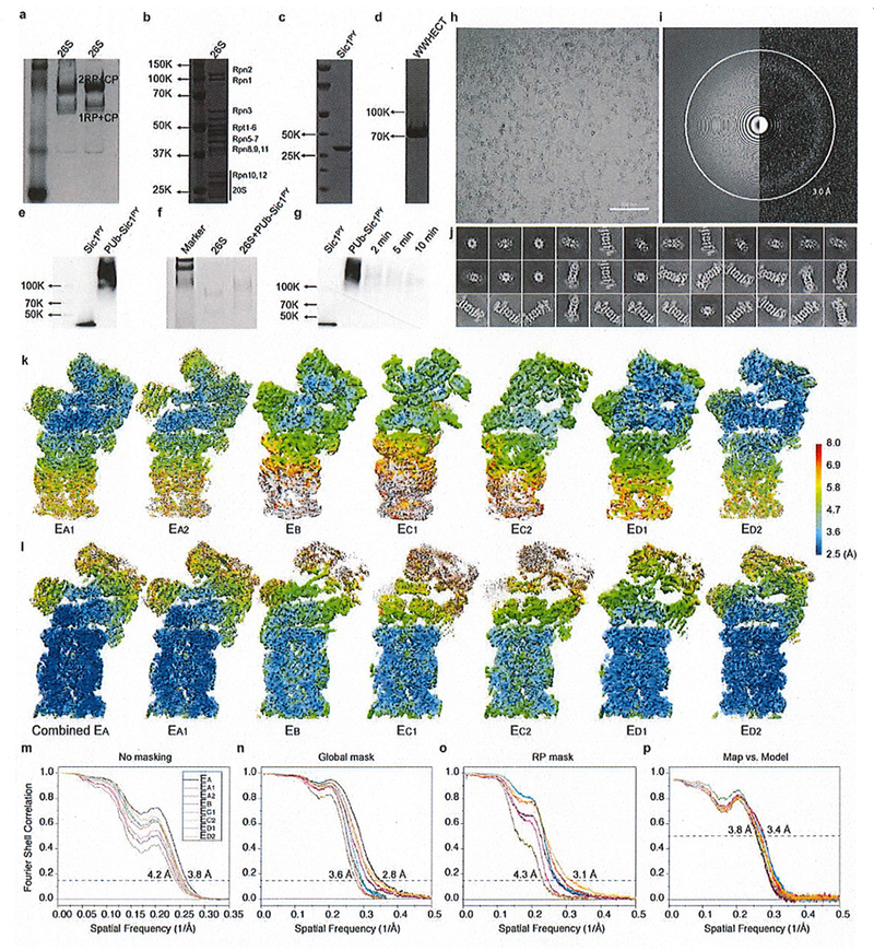
Extended Data Figure 1.
Characterization and structure determination of the substrate-engaged human proteasome.
( a ) Native PAGE analysis of proteasome purified through Superose 6 10/300 GL column. ( b ) SDS-PAGE results of the 26S proteasome after the FPLC. ( c ) SDS-PAGE analysis of the Sic1 PY purified thro...
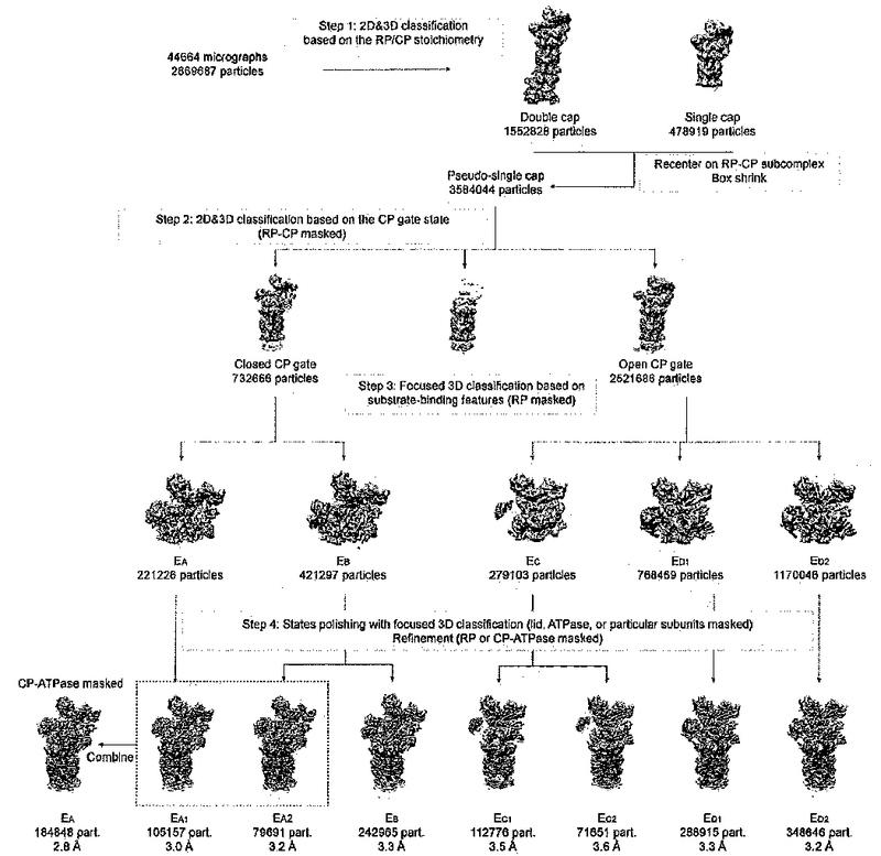
Extended Data Figure 2.
Focused classification to sort out the seven conformational states.
The diagram illustrates the major four steps of our hierarchical focused classification strategy. Further detailed iterations of classification in each step are omitted for clarify.
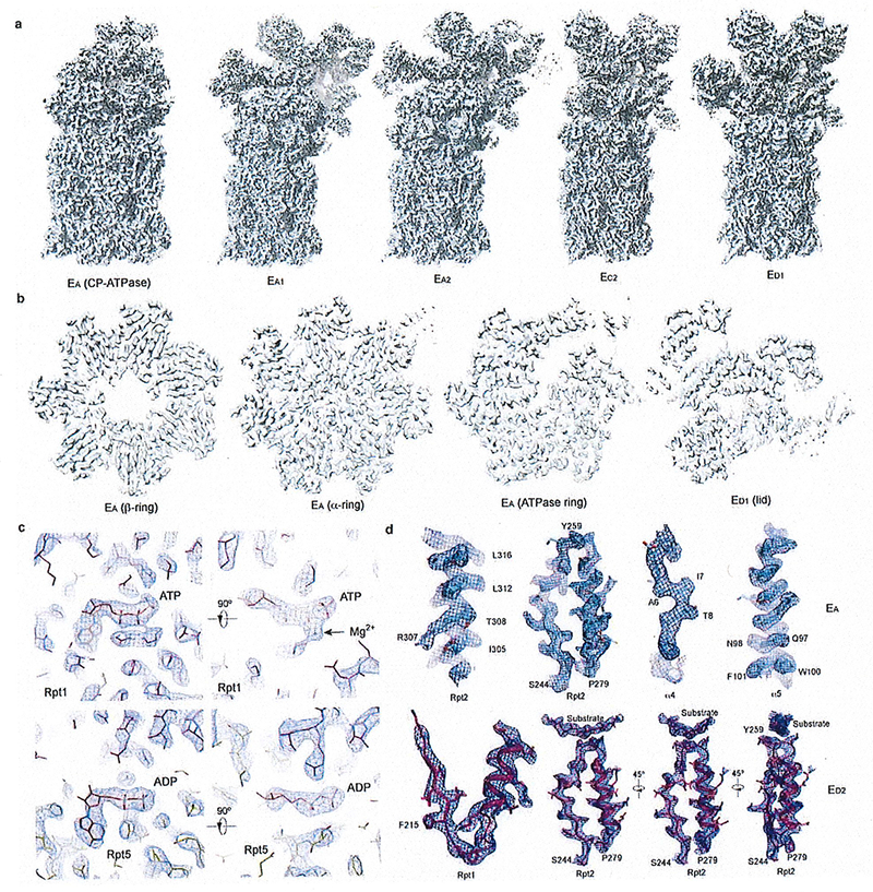
Extended Data Figure 3.
The cryo-EM maps and quality assessment.
( a ) The other five refined cryo-EM maps that are not shown in the main figures. ( b ) Typical central cross-sections in the density maps for each of the four subcomplexes, the lid in state E D1 , th...
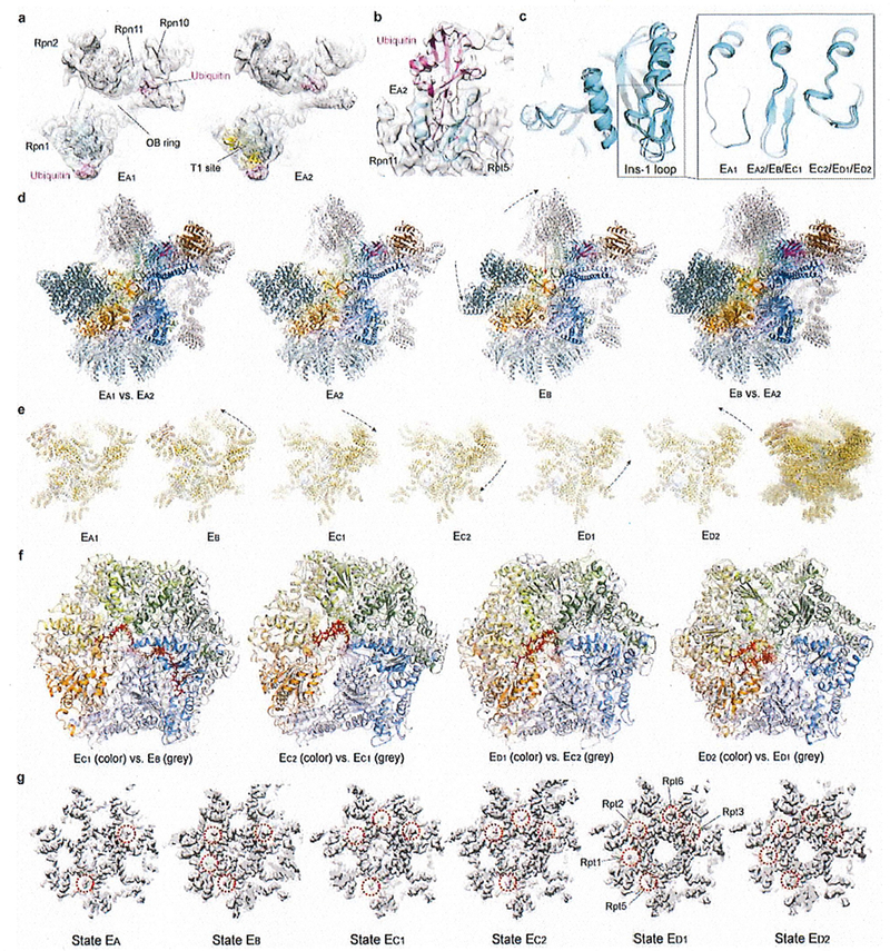
Extended Data Figure 4.
Key structural features and comparisons that help sort out the sequence of the seven conformational states.
( a ) The ubiquitin densities in state E A1 (left) and E A2 (right). The T1 site is labelled by fitting the yellow cartoon representation of the NMR structure (PDB ID 2n3u) of Rpn1 T1 element in compl...
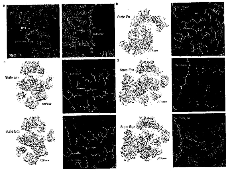
Extended Data Figure 5.
Substrate densities in different states.
( a ) Close-up views of two typical substrate densities observed in the CP chamber in state E A . The left panel shows the substrate density directly contacting the proteolytically active Thr1 in the ...
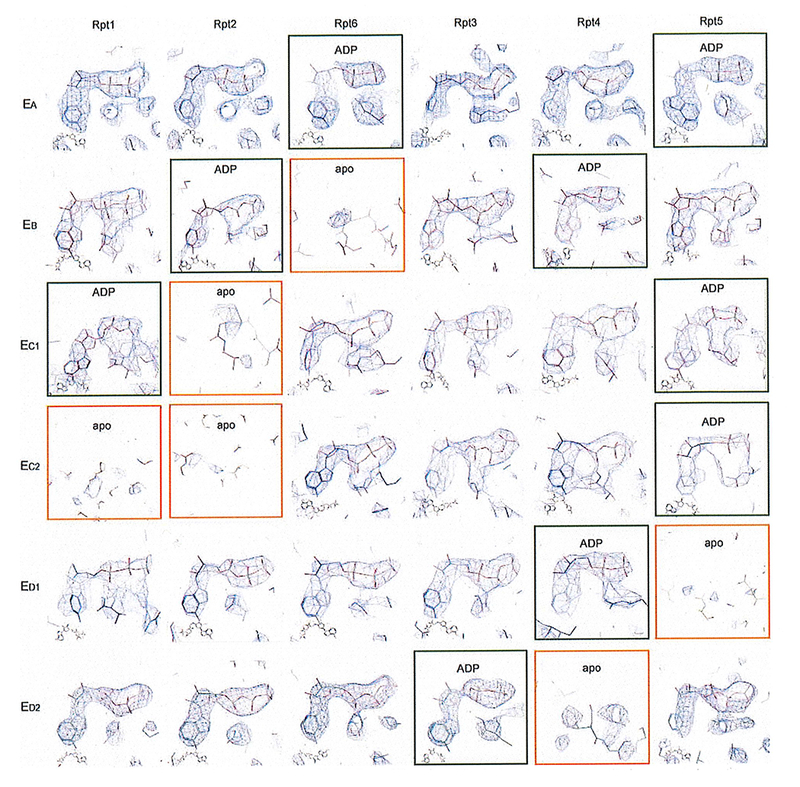
Extended Data Figure 6.
The nucleotide densities in all states.
The nucleotide densities fitting with atomic models are shown with blue meshes. All close-up views were directly screen-copied from Coot 58 after atomic modelling into the density maps without further...
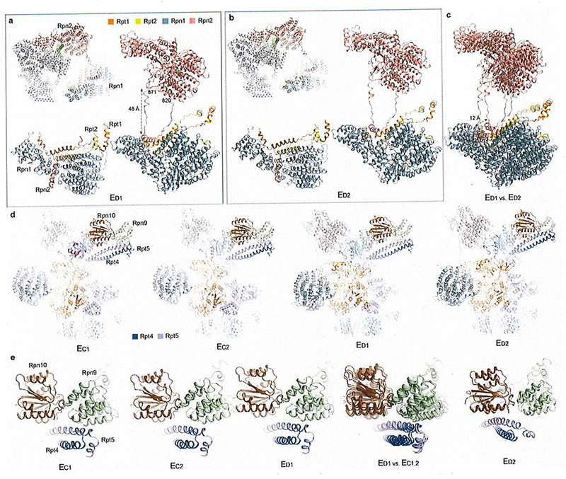
Extended Data Figure 7.
Long-range regulation of the AAA-ATPase by the lid-base interactions.
( a ) and ( b ) The long-range association of the Rpn1-Rpn2 through a looping structure from Rpn2 (residue 820-871) observed in state E D1 ( a ) and E D2 ( b ). ( c ) Comparison of the Rpn1-Rpn2 long-...
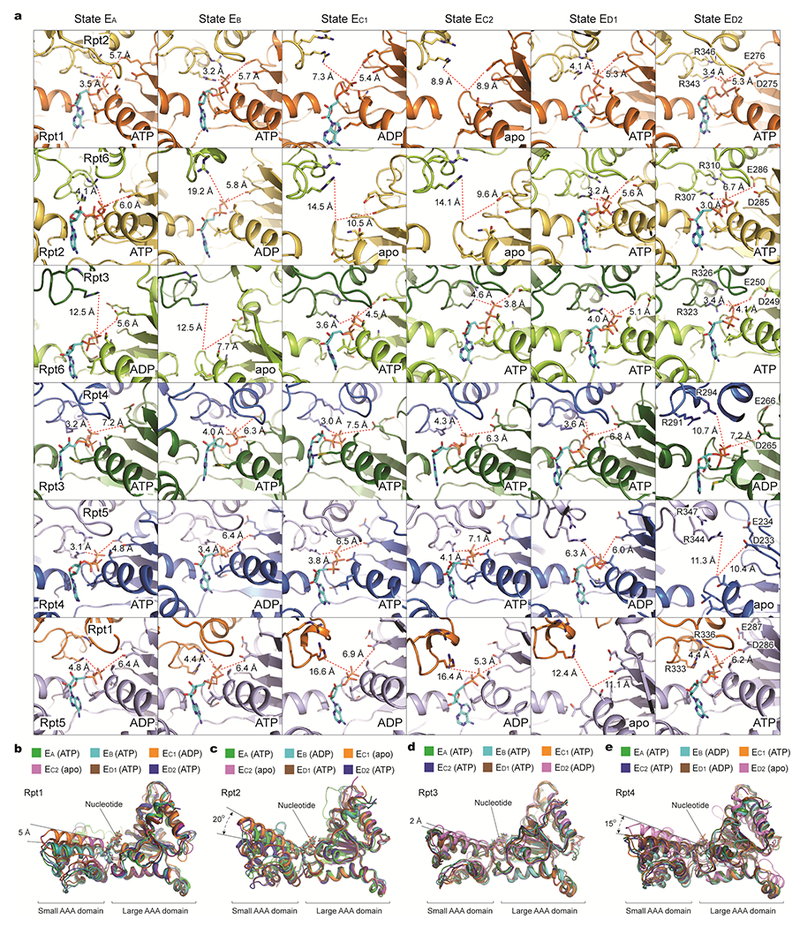
Extended Data Figure 8
Geometries of nucleotide-binding pockets and nucleotide-driven intrasubunit conformational changes of AAA domains.
a , Comparison of the nucleotide-binding pockets of six ATPases in all states illustrates a common pattern in the geometry of the nucleotide-binding sites. Each row shows the geometry of the nucleotid...
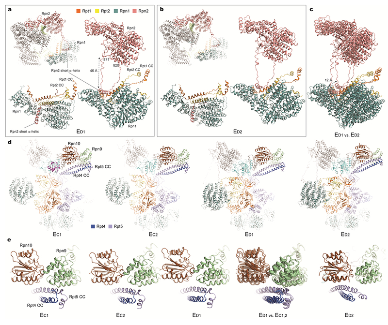
Extended Data Figure 9.
Changes in lid-base interactions are associated with ATP hydrolysis events through long-range allosteric regulation.
a and b , Long-range association between Rpn1 and Rpn2 through a looping structure from Rpn2 (residue 820-871) observed in state E D1 ( a ) and E D2 ( b ). c , Comparison of the Rpn1-Rpn2 long-range a...
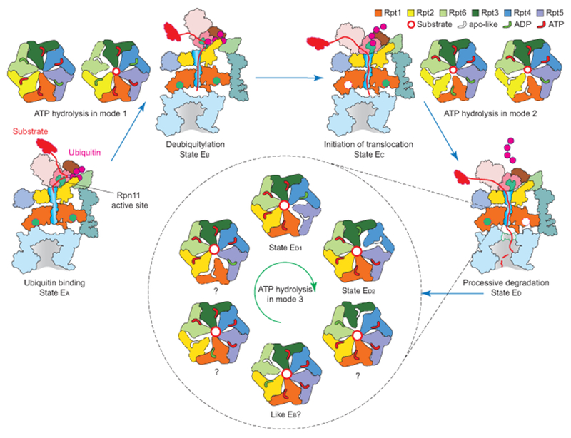
Extended Data Figure 10.
Expanded model of the complete cycle of substrate processing by the human 26S proteasome.
The cartoon summarizes the concept of three principle modes of coordinated ATP hydrolysis observed in the seven states and our proposal of how they regulate the complete cycle of substrate processing ...
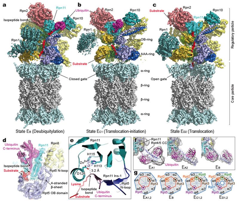
Figure 1.
Cryo-EM structures of the substrate-bound human proteasome in distinct states.
a-c , Cryo-EM density maps of substrate-bound human proteasome in state E B at 3.3 u00c5 ( a ), in state E C1 at 3.5 u00c5 ( b ), and in state E D2 at 3.2 u00c5 ( c ). The Rpt1 density is omitted in a...
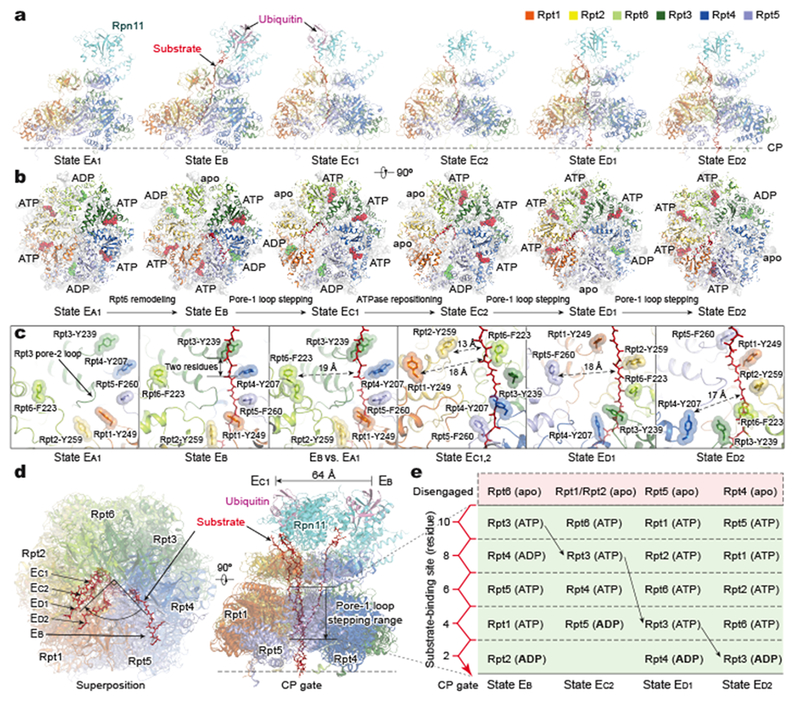
Figure 2.
Dynamic substrate-proteasome interactions.
a , Side views of the ATPase-Rpn11 subcomplex interacting with substrate in five states (E B , E C1,2 and E D1,2 ) in comparison with state E A1 . The substrate is modelled as a polypeptide backbone s...
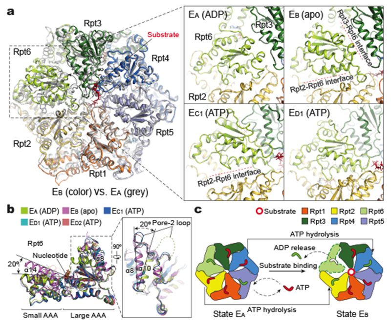
Figure 3.
Structural basis for nucleotide-driven substrate engagement in the AAA-ATPase channel.
a , Superposition of the AAA-ring structures of states E A (grey) and E B (color). The insets show side-by-side comparison of Rpt6 conformations in the four most distant states. Interfacial gaps are m...
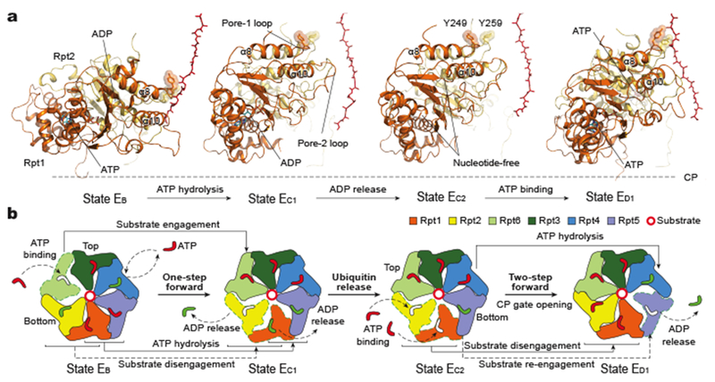
Figure 4.
ATP hydrolysis drives initial three steps of substrate translocation through the AAA-ATPase channel.
a , Side-by-side comparison of the Rpt1-Rpt2 dimer conformations in four sequential states that undergo a complete cycle of ATP hydrolysis and exchange in the Rpt1-Rpt2 dimer. Structures are aligned a...
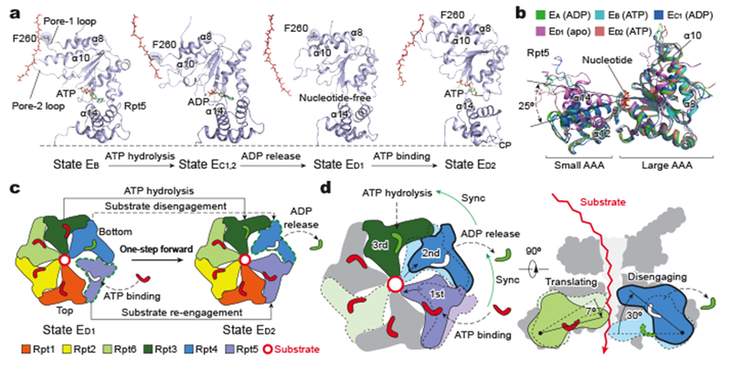
Figure 5.
Mechanism for processive substrate translocation driven by a complete cycle of ATP hydrolysis.
a , Side-by-side comparison of Rpt5 conformations in four sequential states that cover a complete cycle of ATP hydrolysis and exchange in Rpt5. The structures are aligned against the CP to show their ...
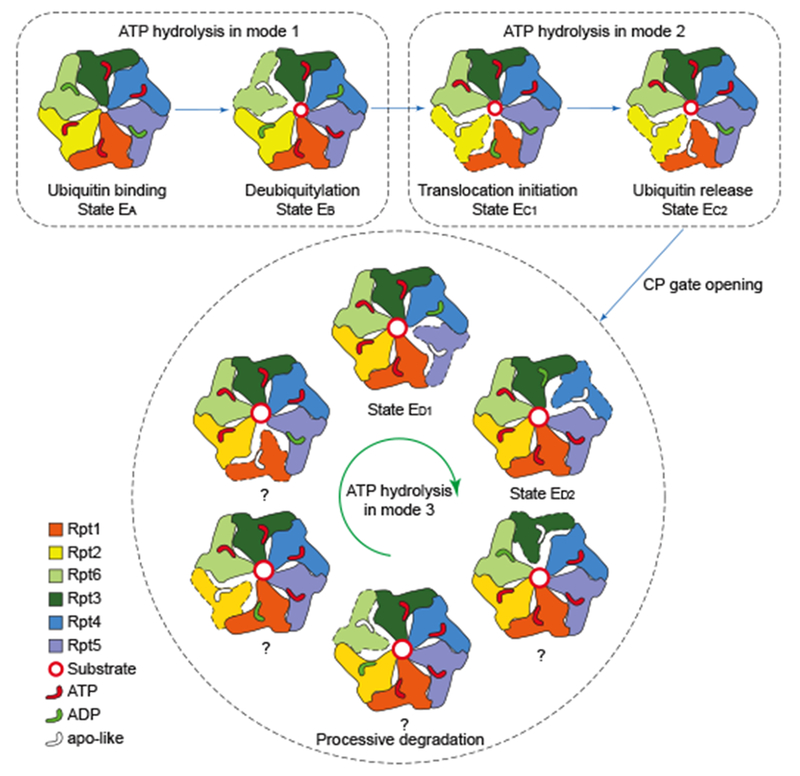
Figure 6.
Model of the complete cycle of substrate processing by the human 26S proteasome.
The cartoon summarizes the concept of three principal modes of coordinated ATP hydrolysis observed in the seven states and our proposal of how they regulate the complete cycle of substrate processing ...
Figure images are served from the NIH/NLM PubMed Central Open Access Subset or Europe PMC; copyright remains with the publishers and authors.
💬 Discussion
0 commentsNo comments yet. Be the first to start a discussion!
Leave a Comment