Abstract
Focal epilepsy involves excessive cortical activity that propagates both locally and distally. Does this propagation follow the same routes as normal cortical activity? We pharmacologically induced focal seizures in primary visual cortex (V1) of awake mice, and compared their propagation to the retinotopic organization of V1 and higher visual areas. We used simultaneous local field potential recordings and widefield imaging of a genetically encoded calcium indicator to measure prolonged seizures (ictal events) and brief interictal events. Both types of event are orders of magnitude larger than normal visual responses, and both start as standing waves: synchronous elevated activity in the V1 focus and in homotopic locations in higher areas, i.e. locations with matching retinotopic preference. Following this common beginning, however, seizures persist and propagate both locally and into homotopic distal regions, and eventually invade all of visual cortex and beyond. We conclude that seizure initiation resembles the initiation of interictal events, and seizure propagation respects the connectivity underlying normal visual processing.Focal cortical seizures result from local and widespread propagation of excitatory activity. Here the authors employ widefield calcium imaging in mouse visual areas to demonstrate that these seizures start as local synchronous activation and then propagate along the connectivity that underlies normal sensory processing.
🔬 Techniques
✨ Fluorophores
🧪 Sample Preparation
🏭 Microscope Brands
🧪 Reagent Suppliers
📷 Detectors
🎨 Filters
💻 Software Details
💾 Data Repositories
🏛️ Research Organizations (ROR)
Affiliated research institutions:
📋 Methods
Procedures
All experimental procedures were conducted according to the UK Animals Scientific Procedures Act (1986). Experiments were performed at University College London, under personal and project licenses released by the Home Office following appropriate ethics review. All data analysis was performed in MATLAB (The MathWorks Inc.). Transgenic lines Emx1::Cre ; CAG::flex-GCaMP3 mice were generated by crossing the following two transgenic lines: Emx1-IRES-Cre , expressing Cre recombinase under the Emx1 promoter (catalog #005628, The Jackson Laboratory); and a reporter Ai38-GCaMP3 line (catalog #014538, The Jackson Laboratory), carrying a floxed copy of the GCaMP3 gene under the strong CAG promoter in the Rosa26 locus. Offspring expressed GCaMP3 in excitatory neurons of the neocortex and hippocampus 24 , 28 . Rasgrf-dCre-CaMKIIa-TTA-TITL-GCaMP6f triple transgenics 27 were generated by breeding Rasgrf-dCre, CamKII-tta and Ai93(TITL-GCaMP6f) mice. Three weeks before imaging, TMP was orally administered for 3 consecutive days to trigger dCre-mediated recombination. With this system, flex-GCaMP6f recombination was induced only in Rasgrf positive neurons, while transcription was further restricted to CaMKIIa expressing neurons that also expressed the transcription factor TTA. As a result, GCaMP6 expression was selective to pyramidal neurons located in layers 2/3 and sparsely in layer 5. Although GCaMP6f allows for the detection of population activity with higher signal to noise ratio than GCaMP3, the cortical activations studied here were so massive that this made little difference. We thus present data obtained with both indicators.
Show full methods section
Procedures
All experimental procedures were conducted according to the UK Animals Scientific Procedures Act (1986). Experiments were performed at University College London, under personal and project licenses released by the Home Office following appropriate ethics review. All data analysis was performed in MATLAB (The MathWorks Inc.). Transgenic lines Emx1::Cre ; CAG::flex-GCaMP3 mice were generated by crossing the following two transgenic lines: Emx1-IRES-Cre , expressing Cre recombinase under the Emx1 promoter (catalog #005628, The Jackson Laboratory); and a reporter Ai38-GCaMP3 line (catalog #014538, The Jackson Laboratory), carrying a floxed copy of the GCaMP3 gene under the strong CAG promoter in the Rosa26 locus. Offspring expressed GCaMP3 in excitatory neurons of the neocortex and hippocampus 24 , 28 . Rasgrf-dCre-CaMKIIa-TTA-TITL-GCaMP6f triple transgenics 27 were generated by breeding Rasgrf-dCre, CamKII-tta and Ai93(TITL-GCaMP6f) mice. Three weeks before imaging, TMP was orally administered for 3 consecutive days to trigger dCre-mediated recombination. With this system, flex-GCaMP6f recombination was induced only in Rasgrf positive neurons, while transcription was further restricted to CaMKIIa expressing neurons that also expressed the transcription factor TTA. As a result, GCaMP6 expression was selective to pyramidal neurons located in layers 2/3 and sparsely in layer 5. Although GCaMP6f allows for the detection of population activity with higher signal to noise ratio than GCaMP3, the cortical activations studied here were so massive that this made little difference. We thus present data obtained with both indicators.
Surgical procedures
Using aseptic techniques, animals were chronically implanted with a thinned skull cranial window under isoflurane anesthesia. 0.05 mL rimadyl (Carprofen 5% w/v) was administered before surgery as an anti-inflammatory and analgesic. During the procedure, eyes were protected with ophthalmic gel (Viscotears Liquid Gel, Alcan) and the body temperature maintained around 37 °C. The animal was anesthetized and mounted in a stereotaxic frame. The scalp over the dorsal skull surface was removed to expose the cranium. The left hemisphere parietal bone was thinned using a scalpel blade. Thinning proceeded until the cancellous layer of the skull, which contains blood vessels, was completely removed. A custom-made stainless-steel head plate with a round imaging chamber (8 mm diameter) was then cemented over the thinned area using dental cement (Superbond). Finally, a small drop of UV cement (Norland Products Inc.) was applied inside the imaging chamber and an 8 mm glass coverslip glued onto the thinned skull region. The cement was cured with an UV LED (390 nm, Thorlabs) for 20 s. The animal was allowed to recover at 37 °C in an incubator and provided with rimadyl in the drinking water (0.1 mL in 100 mL) for the 3 days after the surgery. On the day of LFP recordings, the animal was anaesthetized again and a small skull screw implanted in the contralateral frontal bone, rostral to the cranial window. A silver wire previously soldered to the screw head served as a reference for electrophysiological recordings. After opening a small hole in the cranial window coverslip, a small craniotomy was performed over the target region of V1. The exposed region was finally covered with Kwik-Cast silicone elastomer sealant. The animal was allowed to fully recover before starting the recording session. The typical recording session of epileptiform activity lasted 30–40 min.
Visual stimulation and retinotopic mapping
Visual stimuli were presented on three LCD monitors 25 , positioned 30 cm from the animal, arranged to span 140º in azimuth and 60º in elevation of the visual field contralateral to the imaged hemisphere. For retinotopic mapping, stimuli were contrast-reversing gratings presented inside a rectangular window. Stimulus duration was 5 s, flickering frequency was 2 Hz, and spatial frequency was 0.03 cycles/degree. To measure the preferred azimuth, the rectangular window was 60° high and 30° wide. To measure the preferred elevation, it was 20° high and 140° wide.
Electrophysiology
LFP was recorded with Ag–Cl electrodes in ACSF-filled borosilicate micropipettes (typical tip aperture 2–3 μm, 1–3 MΩ), positioned at 500–600 µm below the dura. To induce epileptiform activity, 10 mM Picrotoxin (Sigma) dissolved in DMSO (Sigma) was added to the recording solution. During these experiments, the pipette was pushed through the dura without applying pressure, to avoid injection of the GABAergic antagonist. In some experiments, we induced epileptiform activity with injections of 100–200 nL of 5M pilocarpine dissolved in DMSO. Because of the viscosity of the solution, the injection pipette was then withdrawn and exchanged with an ACSF-filled borosilicate micropipette to record the LFP. The pressure inside injection pipettes was measured with a differential manometer and kept below 200 mbar. The resistance of the micropipette was monitored to ensure that insertion in the brain did not clog the tip. LFP signals were amplified 1000-fold and high-pass filtered above 0.1 Hz via a Multiclamp 700B differential amplifier (Molecular Devices). Data were digitized at 10 kHz with a Blackrock acquisition system and software. The exposure signal from the camera, the TTL signals from the visual stimulation software and the screen photodiode signal were recorded at the same time to synchronize electrophysiological, imaging and visual stimulation data.
LFP analysis
To identify the start times of interictal events and seizures from the LFP recording we devised a simple supervised event detection method. The LFP trace was resampled at 100 Hz; the start of each event was assigned to the local maxima of the first derivative of the signal that exceeded three standard deviations from baseline; the end of each event was identified when its low frequency envelope returned to baseline. Finally, the results of the automatic detection were inspected visually and events classified as interictal events or seizures. Missed events were manually selected and artifacts removed. Wavelet scalograms of the LFP signal were computed using the wavelet toolbox provided by Torrence and Compo ( atoc.colorado.edu/research/wavelets ). Power spectra and coherence of LFP and fluorescence signals were calculated using the Chronux Toolbox 52 ( http://chronux.org/ ).
Widefield calcium imaging
Imaging experiments were performed under a custom built tandem-lens epifluorescence macroscope 25 , 53 . Excitation light at 480 nm was provided by a blue LED light (465 nm LEX2-B, Brain Vision, band-passed with a Semrock FF01-482/35 filter) and diverted via a dichroic mirror (FF506-Di03, Semrock) into a Leica 1.0× Plan APO (M series, part #10450028) or 1.6× Plan APO objective (M series, part #10450029), which focused the light on the sample. The collected fluorescence was reflected by a second dichroic mirror (FF593-Di03, Semrock), passed through an emission filter (FF01-543/50-25, Semrock), and focused by a second Leica 1.0× Plan APO objective onto the sensor of a sCMOS camera (pco.edge, PCO AG). The camera was controlled by a TTL external trigger synchronized with the visual stimulation. The image acquisition rate was 50 Hz for retinotopic mapping and 70 Hz during imaging of epileptiform activity (except for experiments in the pilocarpine model, imaged at 50 Hz). The nominal spatial resolution of the system was 200 pixel/mm. Imaging was conducted in 20 s long sweeps, interleaved with ~10 s pauses needed to save the data to disk.
Analysis of imaging movies
Widefield movies where first registered using a discrete Fourier transform based subpixel image registration algorithm 54 . The retinotopic mapping and epileptiform activity images where then aligned using the brain vasculature as a reference. Affine transformation was used to find the best alignment. Then we calculated ∆ F / F 0 movies, where the signal for each pixel x at time t was obtained as documentclass[12pt]{minimal} usepackage{amsmath} usepackage{wasysym} usepackage{amsfonts} usepackage{amssymb} usepackage{amsbsy} usepackage{mathrsfs} usepackage{upgreek} setlength{oddsidemargin}{-69pt} begin{document}$$frac{{Delta Fleft( {t,x} right)}}{{{F_0}}} = frac{{Fleft( {t,x} right) - {F_0}left( x right)}}{{{F_0}left( x right)}}$$end{document} Δ F t , x F 0 = F t , x - F 0 x F 0 x Where F 0 was computed as the twentieth percentile of each imaging sweep. Finally, a mask was manually drawn to segment out the visible cortex form the edges of the implant. The map of retinotopy was obtained as previously described 25 . In short, the reversing gratings elicited periodic neural responses that oscillate at twice the frequency of reversal 55 . For each pixel, we measured the power of these second harmonic responses using the Fourier transform of the fluorescent trace. We then fitted a Gaussian position-tuning curve to the amplitude of the responses to visual stimulation at four horizontal positions. The standard deviation for the Gaussian curve model was the one that minimized the least squared error of the fit across pixels. To localize the cortical initiation site of each event, calcium signals were aligned by the start of the electrographic discharge. For each event, pixels were included if they showed Δ F / F increases greater than 60% of the peak Δ F / F reached in the same class of events. The center of mass of the resulting cortical area, calculated over the first 500 ms, was then taken as the site of initiation of epileptiform activity. The average retinotopic position of the focus across animals was 93 ± 16 degrees, confirming our ability to target the medial region of V1. We restricted the analysis to events that were contained for the most part in an imaging sweep. In particular, we included seizures that were imaged for at least 6 s after their start. To assess the slow propagation of seizures, we defined criteria to evaluate when a cortical territory was invaded by the seizing activity. The distribution of maximum florescence levels during seizure was bimodal (Supplementary Fig. 7 ). We considered recruited to the seizure the pixels that exceeded 30% of the peak fluorescence recorded at the focus, which was a good threshold to separate the population of pixels with the highest fluorescence change (Supplementary Fig. 7 ). We then calculated the time it took for a seizure to invade each recruited pixel, measured from the electrographic seizure onset. We called this time ‘delay to seizure invasion’, and we measured it as the time point at which the fluorescence at any recruited pixel reached 60% of its maximum.
Standing wave model
We modeled the fluorescence movies of epileptiform events as standing waves (Fig. 3e ), i.e. as the product of a global time course and a single map (an image) documentclass[12pt]{minimal} usepackage{amsmath} usepackage{wasysym} usepackage{amsfonts} usepackage{amssymb} usepackage{amsbsy} usepackage{mathrsfs} usepackage{upgreek} setlength{oddsidemargin}{-69pt} begin{document}$${rm{Movie = Time course}} times {rm{Map + Residuals}}$$end{document} Movie = Timecourse × Map + Residuals To fit this model (i.e. to minimize the residuals), we used singular value decomposition (SVD), which returns the best least square approximation of a matrix as the sum of standing waves. We obtained the time course and map of the separable model from the first row and first column returned by the SVD. Modeling of the profile of interictal events We modeled the retinotopic profile of activation elicited by interictal events as the dot product of two functions, both dependent on the cortical position x of each ROI. The first function depends on homotopic connectivity, and is a Gaussian falling off with the distance between the retinotopic position R ( x ) of point x and the retinotopic position of the focus, R focus : documentclass[12pt]{minimal} usepackage{amsmath} usepackage{wasysym} usepackage{amsfonts} usepackage{amssymb} usepackage{amsbsy} usepackage{mathrsfs} usepackage{upgreek} setlength{oddsidemargin}{-69pt} begin{document}$$Hleft( {boldsymbol{x}} right) = {{rm e}^{frac{{ - {{left( {Rleft( {boldsymbol{x}} right) - {{boldsymbol{R}}_{{rm{focus}}}}} right)}^2}}}{{2{sigma ^2}}}}}$$end{document} H x = e - R x - R focus 2 2 σ 2 The second function depends on contiguous spread, and is a Gaussian-like function with the numerator raised to the fourth power to give it a flat top as it falls off with the cortical distance from the epileptic focus: documentclass[12pt]{minimal} usepackage{amsmath} usepackage{wasysym} usepackage{amsfonts} usepackage{amssymb} usepackage{amsbsy} usepackage{mathrsfs} usepackage{upgreek} setlength{oddsidemargin}{-69pt} begin{document}$$Cleft( {boldsymbol{x}} right) = left( {a - b} right){{rm e}^{frac{{ - {{left( {{boldsymbol{x}} - {{boldsymbol{x}}_{{rm{focus}}}}} right)}^4}}}{{{lambda ^4}/{rm{ln}}left( 2 right)}}}} + b$$end{document} C x = a - b e - x - x focus 4 λ 4 ∕ ln 2 + b When so parametrized, λ corresponds to the half-width half-maximum of the function. We fitted the parameters σ , λ , R focus , x focus , a , b by least square minimization. Phase analysis of cortical oscillations Movies of cortical seizures were first bandpass filtered between 6 and 11 Hz. Then we computed the analytical representation of the fluorescence time course for each pixel, using the Hilbert transform (MATLAB function ‘hilbert’, Signal Processing Toolbox). The analytical signal S a ( t ) is a representation of a real valued signal f ( t ) in the complex space: documentclass[12pt]{minimal} usepackage{amsmath} usepackage{wasysym} usepackage{amsfonts} usepackage{amssymb} usepackage{amsbsy} usepackage{mathrsfs} usepackage{upgreek} setlength{oddsidemargin}{-69pt} begin{document}$${S_a}left( t right) = fleft( t right) + iH(f)(t) = A(t){{rm e}^{ivarphi (t)}}$$end{document} S a t = f t + i H ( f ) ( t ) = A ( t ) e i φ ( t ) Its real part is f ( t ), the fluorescence signal, while its imaginary part is H ( f )( t ), the Hilbert transform of f ( t ). When expressed in polar form, the analytical signal S a ( t ) has a straightforward interpretation: the modulus A ( t ) represents the instantaneous amplitude, or envelope, of the oscillation; the angle φ ( t ) represents the instantaneous phase of the oscillation.
Behavioral data
The eye contralateral to the imaged cortex was imaged with a monochrome CCD camera (DMK 21BU04.H, The Imaging Source), equipped with a macro zoom lens (MVL7000—18–108 mm EFL, f/2.5, Thorlabs). Illumination to the eye was provided by two infrared LEDs (850 nm, Mightex, powered by an SLC-SA/AA LED controller, Mightex). An infrared filter (700 nm high-pass, #092, The Imaging Source) was applied to the camera objective to shield it from stray light. Eye imaging movies were processed with custom software to extract eye movements, pupil dilations and blinks. The running behavior was measured using a rotary encoder (Kübler 05.2400.1122.0100) that tracked the revolutions of the cylindrical treadmill. The angular displacement was first converted into angular speed and then into linear speed based on the diameter of the treadmill. Both the rotary encoder signal and the frame time stamps from the eye-tracking camera were acquired using a data acquisition board (National Instruments, PCIe-6323). The same board acquired a copy of the exposure signal from the imaging camera, the TTL signals from the visual stimulation software and the screen photodiode signal: such signals were used to align imaging, electrophysiological and behavioral recordings. Statistical information Data were tested for normality before choosing the appropriate statistical test. All the statistical tests used were 2-tailed test. The significance of linear regression models was tested with the F-statistic against the null hypothesis of a constant model. p = 0.05 was assumed as the threshold for statistical significance.
Code availability
All the relevant code is available from the authors upon request. Representative code can be found at www.ucl.ac.uk/cortexlab/data .
Data and code availability
All the relevant data are available from the authors upon request. An example data set can be found at www.ucl.ac.uk/cortexlab/data .
Procedures
All experimental procedures were conducted according to the UK Animals Scientific Procedures Act (1986). Experiments were performed at University College London, under personal and project licenses released by the Home Office following appropriate ethics review. All data analysis was performed in MATLAB (The MathWorks Inc.).
Surgical procedures
Using aseptic techniques, animals were chronically implanted with a thinned skull cranial window under isoflurane anesthesia. 0.05 mL rimadyl (Carprofen 5% w/v) was administered before surgery as an anti-inflammatory and analgesic. During the procedure, eyes were protected with ophthalmic gel (Viscotears Liquid Gel, Alcan) and the body temperature maintained around 37 °C. The animal was anesthetized and mounted in a stereotaxic frame. The scalp over the dorsal skull surface was removed to expose the cranium. The left hemisphere parietal bone was thinned using a scalpel blade. Thinning proceeded until the cancellous layer of the skull, which contains blood vessels, was completely removed. A custom-made stainless-steel head plate with a round imaging chamber (8 mm diameter) was then cemented over the thinned area using dental cement (Superbond). Finally, a small drop of UV cement (Norland Products Inc.) was applied inside the imaging chamber and an 8 mm glass coverslip glued onto the thinned skull region. The cement was cured with an UV LED (390 nm, Thorlabs) for 20 s. The animal was allowed to recover at 37 °C in an incubator and provided with rimadyl in the drinking water (0.1 mL in 100 mL) for the 3 days after the surgery. On the day of LFP recordings, the animal was anaesthetized again and a small skull screw implanted in the contralateral frontal bone, rostral to the cranial window. A silver wire previously soldered to the screw head served as a reference for electrophysiological recordings. After opening a small hole in the cranial window coverslip, a small craniotomy was performed over the target region of V1. The exposed region was finally covered with Kwik-Cast silicone elastomer sealant. The animal was allowed to fully recover before starting the recording session. The typical recording session of epileptiform activity lasted 30–40 min.
Electronic supplementary material Supplementary Information Peer Review File Supplementary Movie 1 Supplementary Movie 2 Supplementary Movie 3 Supplementary Movie 4
📊 Figures

Fig. 1
Testing hypotheses for cortical seizure propagation with simultaneous imaging, recordings and behavioral measurements in the awake mouse. a Cartoon of mouse visual cortex showing six visual areas in t...
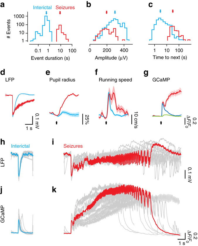
Fig. 2
Neural and behavioral signatures of seizures and interictal events. a Distribution of the duration of interictal events ( blue ) and seizures ( red ). Arrows indicate the medians of each distribution....

Fig. 3
Interictal events and seizures start as standing waves, and seizures subsequently propagate widely across cortex. a Frames obtained through GCaMP imaging in a representative interictal event (the one ...

Fig. 4
Interictal events and early seizures engage both contiguous spread and homotopic connectivity. a Average spatial profile of interictal events measured in one mouse, obtained by averaging the maximum p...

Fig. 5
Seizure propagation recruits homotopic regions of cortex. a Frames imaged in a representative seizure. Labels indicate time from seizure onset, and cartoon electrode indicates the site of Ptx injectio...

Fig. 6
Homotopic propagation of 6u201311u2009Hz oscillations during seizures. a LFP recording of the seizure in Fig. 5a , bandpass filtered between 6 and 11u2009Hz. Highlighted in black is an epoch of cohere...
Figure images are served from the NIH/NLM PubMed Central Open Access Subset or Europe PMC; copyright remains with the publishers and authors.
💬 Discussion
0 commentsNo comments yet. Be the first to start a discussion!
Leave a Comment