Abstract
The ever-increasing speed and resolution of modern microscopes make the storage and post-processing of images challenging and prevent thorough statistical analyses in developmental biology. Here, instead of deploying massive storage and computing power, we exploit the spherical geometry of zebrafish embryos by computing a radial maximum intensity projection in real time with a 240-fold reduction in data rate. In our four-lens selective plane illumination microscope (SPIM) setup the development of multiple embryos is recorded in parallel and a map of all labelled cells is obtained for each embryo in <10 s. In these panoramic projections, cell segmentation and flow analysis reveal characteristic migration patterns and global tissue remodelling in the early endoderm. Merging data from many samples uncover stereotypic patterns that are fundamental to endoderm development in every embryo. We demonstrate that processing and compressing raw image data in real time is not only efficient but indispensable for image-based systems biology.
🔬 Techniques
🧬 Organisms
💻 Software
✨ Fluorophores
🧪 Sample Preparation
🏭 Microscope Brands
🔴 Lasers
📷 Detectors
💻 Software Details
🏛️ Research Organizations (ROR)
Affiliated research institutions:
📋 Methods
SPIM hardware
The four-lens SPIM setup consists of four identical water-dipping Olympus UMPLFLN 10x/0.3 objectives, two for illumination and two for detection. The sample chamber was custom-made from acrylic with four openings sealed with rubber o-rings. The sample position and the light sheets are monitored with a webcam through a glass window on the bottom of the chamber. Two Toptica iBeam smart (488 nm, 200 mW) lasers were externally triggered for alternating double-sided illumination. Each beam was guided with an optical fibre onto a continuously running galvanometric mirror (1 kHz, EOPC) for even fluorescence illumination (multidirectional SPIM 17 ). Light sheets were generated with cylindrical lenses and projected with telescopes and the illumination objective lenses onto the common focal plane of both detection lenses. The average excitation power in the entire object plane was ~6 mW per arm. The focal planes of the two detection objectives were imaged onto two Andor Zyla sCMOS cameras through emission filters (Chroma ET BP525/50). Both cameras were precisely aligned via a focusable tube lens and an adjustable mirror to acquire images from the same focal plane, which were streamed to separate computers. The sample was moved and rotated with three motorized linear stages (M-404.1PD/6PD, M-112.1DG) and one rotational stage (M-660.55, Physik Instrumente) using a custom-made software ( Supplementary Methods ). Zebrafish Zebrafish were handled in accordance with EU directive 2011/63/EU as well as the German Animal Welfare Act. The transgenic zebrafish line Tg(sox17:EGFP) 13 18 was used for visualizing endodermal cells during gastrulation. Embryos were collected after fertilization and incubated at 32 °C to speed up development while the temperature during imaging was kept constant at 24 °C. For morphant experiments, embryos were injected with 10 ng of cxcr4a morpholino (5′-AGACGATGTGTTCGTAATAAGCCAT-3′) at the 1-cell stage 12 .
Show full methods section
SPIM hardware
The four-lens SPIM setup consists of four identical water-dipping Olympus UMPLFLN 10x/0.3 objectives, two for illumination and two for detection. The sample chamber was custom-made from acrylic with four openings sealed with rubber o-rings. The sample position and the light sheets are monitored with a webcam through a glass window on the bottom of the chamber. Two Toptica iBeam smart (488 nm, 200 mW) lasers were externally triggered for alternating double-sided illumination. Each beam was guided with an optical fibre onto a continuously running galvanometric mirror (1 kHz, EOPC) for even fluorescence illumination (multidirectional SPIM 17 ). Light sheets were generated with cylindrical lenses and projected with telescopes and the illumination objective lenses onto the common focal plane of both detection lenses. The average excitation power in the entire object plane was ~6 mW per arm. The focal planes of the two detection objectives were imaged onto two Andor Zyla sCMOS cameras through emission filters (Chroma ET BP525/50). Both cameras were precisely aligned via a focusable tube lens and an adjustable mirror to acquire images from the same focal plane, which were streamed to separate computers. The sample was moved and rotated with three motorized linear stages (M-404.1PD/6PD, M-112.1DG) and one rotational stage (M-660.55, Physik Instrumente) using a custom-made software ( Supplementary Methods ). Zebrafish Zebrafish were handled in accordance with EU directive 2011/63/EU as well as the German Animal Welfare Act. The transgenic zebrafish line Tg(sox17:EGFP) 13 18 was used for visualizing endodermal cells during gastrulation. Embryos were collected after fertilization and incubated at 32 °C to speed up development while the temperature during imaging was kept constant at 24 °C. For morphant experiments, embryos were injected with 10 ng of cxcr4a morpholino (5′-AGACGATGTGTTCGTAATAAGCCAT-3′) at the 1-cell stage 12 .
Sample embedding
Low-melting agarose (1.5%) solution was prepared in E3 medium and maintained at 37 °C. At 30% epiboly stage, embryos with chorion were transferred into low-melting agarose and sucked into a cleaned FEP tube 6 (inner diameter: 2.0 mm, wall thickness: 0.5 mm), using a syringe and needle. The embryos are positioned on top of each other with minimum gap between them. The agarose was allowed to solidify at room temperature for 5 min and the FEP tube was mounted on the stage, dipping from the top into the sample chamber filled with E3 medium for time-lapse acquisition.
Time-lapse acquisition
The zebrafish embryo was moved along the detection axis through the alternating light sheets to acquire a z -stack of 402 planes. The two cameras were triggered simultaneously by the stage every 2 μm, acquiring one projection for each combination of illumination side and camera. The laser light was triggered when the entire chip was exposed avoiding any artefacts due to the rolling shutter. The sample was then rotated by 45° to acquire a second view, generating a total of eight projections at each time point. These steps were repeated at an interval of 30 s for a period of 12 h. In parallel, the eight projections were fused using nonlinear blending to generate a single data set based on the transformations pre-calculated with the bead sample. For imaging multiple samples in parallel, we omitted the rotation of the sample. Instead, a z -stack was acquired for one embryo and the stage translated the tube along the y axis to position the next embryo in front of the objective lenses. By repeating this, a time point is acquired for each sample and the stage moves back to bring the first embryo in the field of view. This entire process is repeated for time-lapse acquisition of multiple samples. To confirm that the laser light does not induce any developmental defects we compared two embryos that were embedded in the same tube. One was imaged for 12 h, whereas the other one was not exposed to any laser light. We found no morphological differences ( Supplementary Fig. S9 ) and both embryos were raised without defects. We also performed a timelapse with reduced speed, in which an embryo was imaged only every 15 min. We could not observe any difference to an embryo that was imaged every 30 s, as usually done in single-sample experiments ( Supplementary Movie 15 ). At the end of an experiment we captured another transmission stack to verify that the initially fitted sphere model had been valid during the course of the entire timelapse. Registration of time points When the embryonic axis forms towards the end of gastrulation, the embryo inside the chorion turns by 90°. To separate this global movement from local cell movements, images of consecutive time points were registered rigidly ( Supplementary Movies 4 and 5 ). For this purpose, the Fuller projection was calculated at each time point and smoothed using a Gaussian kernel with σ =1.5. ImageJ’s MaximumFinder plugin was used to detect local image maxima with an intensity tolerance of 10, which detected the centres of the majority of cells. The best rigid transformation between the cell centres of consecutive time points was then estimated using the Iterative Closest Point algorithm 21 22 .
Real-time processing
The software for radial projection can be applied both in real-time (images obtained directly from the camera) and post-processing (images read from the hard drive). To ensure that our software is working correctly we performed a time-lapse experiment with reduced temporal resolution, allowing us to save the raw image data. We then calculated radial projections post-processing and compared it to the raw data for consistency. Using offline data we found that our processing framework can deal with data rates of up to 250 f.p.s. Acquisition computers used for real-time processing were two Dell T7500 workstations (2 × 2.3 GHz Dual-Core, 60 GB RAM). As soon as projections were created on the acquisition computers, they are copied via a gigabit Ethernet connection to a Mac Pro workstation (2 × 2.26 GHz Quad-Core Intel Xeon, 32 GB RAM) for fusion, registration and map projections. The source code for radial maximum projection, fusion, registration and map projection is publicly available ( Supplementary Software 1 ).
2D map projections
Generally, map projections aim to find a planar projection of a spherical surface such that angles, areas, distances and shapes are preserved. However, it is impossible to meet all of these requirements in a single projection, and therefore, many different types of projections have been invented. Applied to our biological data, the distortions introduced by a particular projection type influence the interpretation of the data, so that the choice for a projection needs to be taken with care. In our application we are quantifying and visualizing cellular movement of the endoderm. For analysing directionality of cell flow, the Mercator projection is ideal as it is conformal, that is, angle-preserving. To study the density of cells, area-preserving projections such as the Bonne or Gall-Peters projections are preferred. Finally, for the visualization of the global cellular flow projections reducing the overall shape distortions are preferable, such as the Fuller and Winkel Tripel projections. Map projections are ideal for visualization, as they depict the entire surface in a single 2D image. For further processing and quantification, however, we chose to use the raw vertex data where possible to avoid distortions. The final projections depict the data in polar coordinates instead of Cartesian coordinates. This way slight size differences between embryos are eliminated and their cellular pattern can be directly compared. In our projections, the commonly used scale bar is not applicable any more. The radius of the sphere provides the necessary information about the dimensions of the embryo. Distortions in the Mercator projection resulting from an incorrectly determined centre or a non-spherical embryo have been quantified ( Supplementary Fig. S10 ) and would allow us to identify and reject such data. A Java library that was originally designed for cartography and implements all common map projections ( http://www.jhlabs.com/java/maps/proj ) was used to map the spherical data on to 2D planar images.
Cell segmentation and tracking
The projected raw images were processed with a Retinex filter 23 to enhance the local image contrast and reduce spatial in homogeneity in image intensities. A total-variation filter was applied to reduce noise while preserving image structures 24 . Both filters were implemented in C++. Cells were detected in the Mercator projections by applying an active contours method, which allowed us to control spatial regularity of detected cell shapes 25 . An adapted size constraint was used to eliminate small, noisy artefacts, where the local area distortions of the mapping were explicitly taken into account by using an adaptive size constraint with respect to the latitude position of each cell. Each cell was tagged with an individual ID with connected component labelling. Dense deformation fields between consecutive frames were obtained by applying a fast fluid image registration 26 . Cells were finally tracked by propagating the detected cell masks with the obtained flow fields from the registration and subsequent consistency check 27 ( Supplementary Methods ). All methods were implemented in Mathematica v8.0 (Wolfram Research) except for the registration and raw segmentation (C++).
Feature quantification and visualization
All relevant features were evaluated either in the suitable projections or in spherical coordinates: directions of cell migration on the conformal Mercator map, densities on the area-preserving Bonne projection and distances were evaluated as great circle distances in the original spherical coordinates. Overlays of cell tracks from multiple samples were computed after alignment of all samples to the position of the DFCs at tailbud stage. Streamline plots, that is, lines of flow that are tangential to the flow vectors at each point, were computed from a static global flow field obtained by estimating the mean flow direction at each point in space. Flow directions were estimated by computing the average direction (vector sum of normalized directions) of trajectory samples (length n =10 data points) in a spatial box around each point. The margin around the DFCs was analysed by calculating the distance of each cell from the DFC and subsequent binning of the obtained distances. Radial histograms from each time point were concatenated to produce the kymographs ( Supplementary Fig. S8 ). The radii of the margin around the DFC were estimated by the 0.1 quantile of the annular distribution for each time point. The planar visualizations were computed in Mathematica, and volume renderings were done with custom Python scripts and Blender ( http://www.blender.org/ ). Analysis of movies (fluid registration, cell detection, tracking and visualization) was done on a MacBook Pro with 8GB of RAM and a QuadCore 2.3 GHz Intel Core i7. To further speedup post-processing and analysis of multi-sample data, several movies were processed in parallel on a compute server with 24 Intel Xeon CPUs running at 2.67 GHz.
Supplementary Material Supplementary Figures, Methods and References Supplementary Figures S1-S10, Supplementary Methods and Supplementary References Supplementary Software 1 Source code for radial maximum projection, fusion, registration and map projection. Supplementary Movie 1 Illustration of multi-view acquisition. During acquisition, the sample is moved through the light sheet that is generated alternately by two illumination lenses (top and bottom). Each of the two detection lenses (left and right) captures one hemisphere. Indicated are the parts of the sample that are imaged under ideal conditions. A second view is acquired after turning the sample by 45°. The movie demonstrates the interplay of illumination, detection and sample orientation to cover the entire embryo with uniform image quality. Supplementary Movie 2 Flattening the embryo. The entire embryo is assembled from eight parts, each of which is imaged best by a specific combination of illumination, detection and sample orientation. This movie shows how the different parts get mapped onto a 2D plane, in this case using the Gall-Peters projection. The four colors highlight the parts that are acquired with two cameras for both orientations of the sample. Supplementary Movie 3 Illustration of real-time projection. While the sample is moved through the light sheet the projection is updated in real-time. A specific combination of illumination side, detection camera and rotation angle fills in the values for one of the eight parts (see also Supplementary Movie 1). Once all eight parts are obtained, they are fused via non-linear blending. The Mercator projection is shown here for illustration, while the actual real-time projection is performed using sphere vertices instead of a regular pixel grid. Supplementary Movie 4 : The benefit of registration (orthogonal projection). Two consecutive images are aligned with each other to eliminate any global movement of the embryo itself and to preserve local cell movements. The data is then arranged such that the axis of the embryo lands in the middle of the image at the final time point. This movie compares an unregistered (left) and registered (right) projection. An orthogonal projection is used here since it provides the most intuitive illustration of global rotations to the human eye. Supplementary Movie 5 The benefit of registration (Mercator projection). This movie demonstrates the effect of registration on the Mercator projection (same data as in Supplementary Movie 3). Supplementary Movie 6 Overview of different projection types. The same data set is shown using different map projections: (a) Winkel Tripel and (b) Fuller (distortion reducing), (c) Mercator (angle-preserving), (d) Bonne (area-preserving) and (e) orthogonal projection. Supplementary Movie 7 Projected data of a wildtype embryo. Focusing on the first hours of development, this movie shows a Winkel Tripel projection of the raw registered data of a wild-type embryo in full temporal resolution, acquired every 30 s. Frame rate: 30 frames per second (fps), i.e. 1 second in the movie corresponds to 15 minutes experimental time. Supplementary Movie 8 Multi-layer projection of a wildtype embryo. In order to visualize the invagination of endoderm post gastrulation, multilayer projection was generated. The movie shows different radial layers in different colors to visualize the 3D information in a single image. Frame rate: 15 frames per second (fps), i.e. 1 second in the movie correspond to 15 minutes experimental time. Supplementary Movie 9 Multi-sample time-lapse of wildtype embryos. Four wildtype embryos were mounted in the same FEP tube and imaged simultaneously for 12h. This movie shows the raw registered data on a Mercator projection, acquired every minute. Frame rate: 20 frames per second (fps), i.e. 1 second in the movie correspond to 20 minutes experimental time. Supplementary Movie 10 Cell segmentation. This movie demonstrates the results of cell detection and tracking. A wild-type dataset is shown in Mercator projection. Detected cell masks are indicated as colored overlay on the original image sequence. Individual cells are shown in different colors. Cell detection starts at 1 h, when the GFP signal is bright enough to be reliably detected and ends at 5 h, when individual cells are no longer discernible around the dorsal midline. Frame rate: 30 fps, i.e. 1 second in the movie corresponds to 15 minutes experimental time. Supplementary Movie 11 Orientation of cell movements in a wildtype embryo. This movie shows the orientation of cell movement in a wildtype embryo over time. The Mercator projection is chosen to preserve angles. Cell tracks are shown for each detected cell. Color scale indicates the unsigned angle between the cell track (end-to-end vector) and the horizontal axis (dorsal midline) from blue (0) to red (p/2). Cell detection begins at 1h, when the GFP signal is bright enough to be reliably detected and ends at 5h, when individual cells are no longer discernible around the dorsal midline. Frame rate: 60 fps, i.e. 1 second in the movie corresponds to 30 minutes experimental time. Supplementary Movie 12 Projected data of a cxcr4a morphant embryo. Focusing on the first hours of development, this movie shows a Winkel Tripel projection of the raw registered data of a morphant embryo in full temporal resolution, acquired every 30 s. Frame rate: 30 fps, i.e. 1 second in the movie corresponds to 15 minutes experimental time. Supplementary Movie 13 Orientation of cell movements in a cxcr4a morphant embryo. This movie shows the orientation of cell movement in a cxcr4a morphant embryo over time. The Mercator projection is chosen to preserve angles. Cell tracks are shown for each detected cell. Color scale indicates the unsigned angle between the cell track (end-to-end vector) and the horizontal axis (dorsal midline) from blue (0) to red (p/2). Cell detection begins at 1 h, when the GFP signal is bright enough to be reliably detected and ends at 5 h, when individual cells are no longer discernible around the dorsal midline. Frame rate: 60 fps, i.e. 1 second in the movie corresponds to 30 minutes experimental time. Supplementary Movie 14 Comparison of cell densities in a wildtype and cxcr4a morphant embryo. This movie compares the cell density distribution in a wildtype and cxcr4aMO embryo over time. The sinusoidal Bonne projection is chosen to preserve areas. The color code for densities range from blue (0) to white (>8 cells/1000 μm2). Frame rate: 60 fps, i.e. 1 second in the movie corresponds to 30 minutes experimental time. Supplementary Movie 15 Wildtype embryos imaged at different rates. To check for the phototoxic effect on embryos due to high speed imaging, two wildtype embryos were imaged at different intervals. One imaged every 30 seconds and the other was sampled only every 15 minutes. This movie compares the dynamics of the two on an orthogonal projection.
📊 Figures
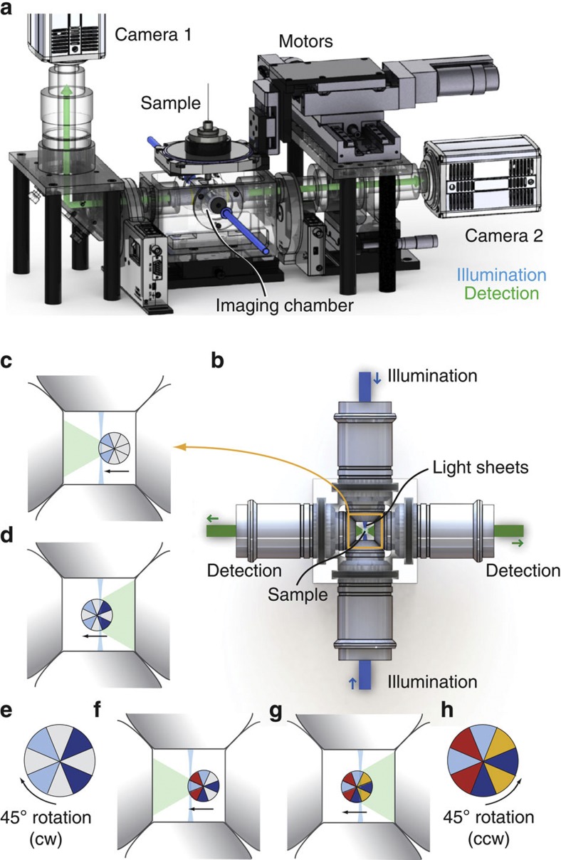
Figure 1
Four-lens SPIM setup and image acquisition.
( a ) Schematic of the central unit of the four-lens SPIM setup. The sample dips into the medium-filled imaging chamber from the top. It is held and moved by a fast rotational stage and three linear m...
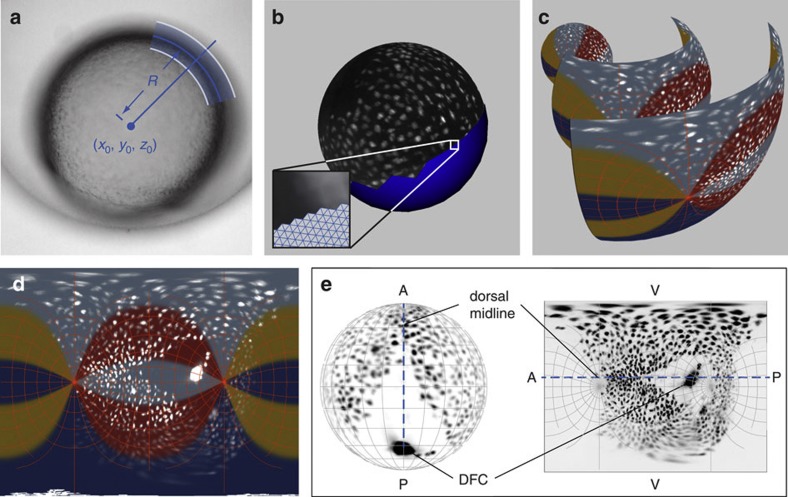
Figure 2
Spherical projection and real-time processing.
( a ) A sphere is fitted to a series of transmission images of a zebrafish embryo. The coordinates of the centre ( x 0 , y 0 , z 0 ) and the radius ( R ) are determined. A shell of 140u2009u03bcm thic...
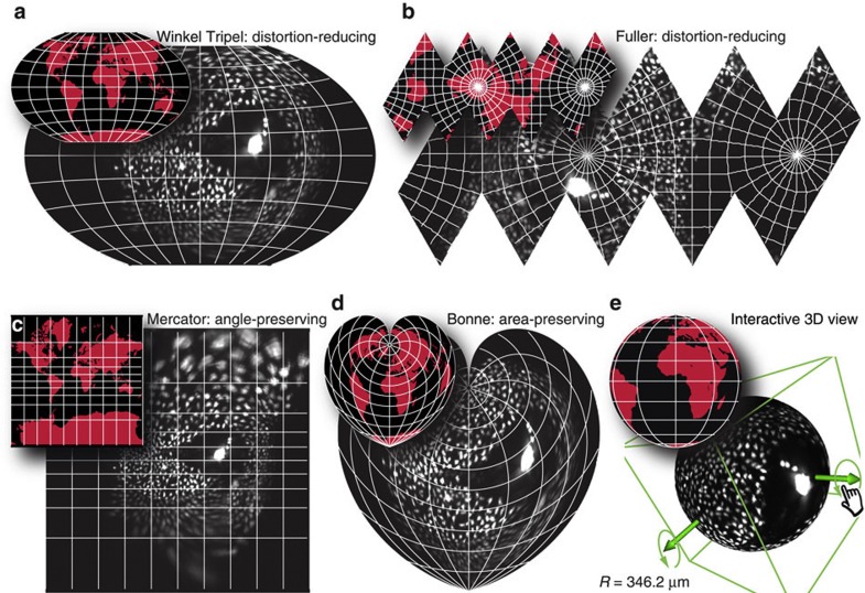
Figure 3
Map projections to visualize the entire endoderm.
Various map projections are available to quantify different parameters and visualize patterns of cell organization ( Supplementary Movie 6 ). ( a , b ) Winkel Tripel and Fuller projections show little...
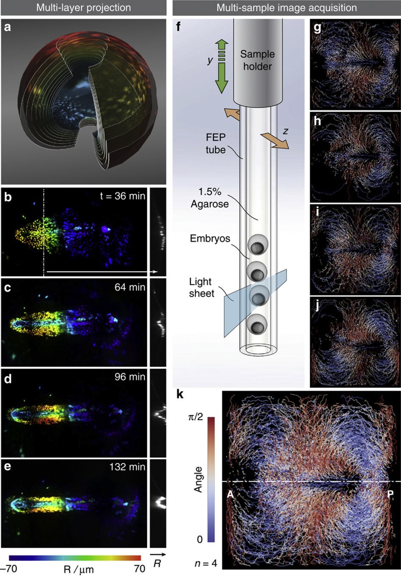
Figure 4
Multi-layer projections and multi-sample acquisition.
A multi-layer projection is created to capture the radial movement of cells during late gastrulation. ( a ) Rendering of a radial multi-layer projection, cut open to show the different layers, which a...
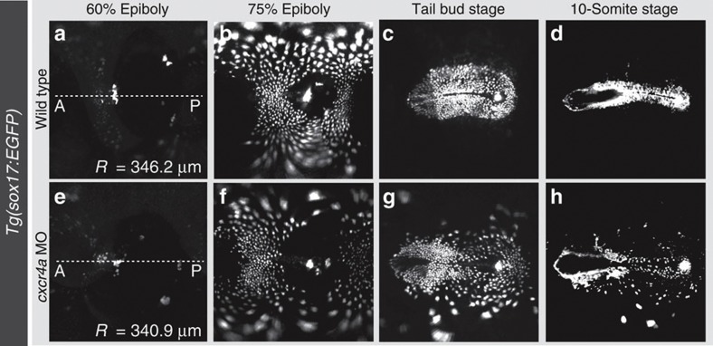
Figure 5
Visualizing endoderm cell dynamics in wild-type and crxcr4a morphant embryos.
Time-lapse images of the entire developing endoderm in Mercator projections. Tg(sox17:EGFP) line was used to visualize the endoderm from 60% epiboly to 10-somite stage ( a u2013 d ) in wild type and (...
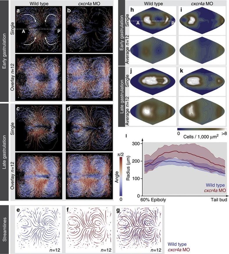
Figure 6
Quantification of endoderm cell dynamics reveals conserved flow patterns.
For quantitative analysis, movies were split into early (60u201375% epiboly) and late gastrulation (75% epiboly, tail bud). ( a u2013 d ) Orientation of cell migration ( a , c ) for wild type and ( b ...
Figure images are served from the NIH/NLM PubMed Central Open Access Subset or Europe PMC; copyright remains with the publishers and authors.
💬 Discussion
0 commentsNo comments yet. Be the first to start a discussion!
Leave a Comment