Abstract
Single cell segmentation is a critical and challenging step in cell imaging analysis. Traditional processing methods require time and labor to manually fine-tune parameters and lack parameter transferability between different situations. Recently, deep convolutional neural networks (CNN) treat segmentation as a pixel-wise classification problem and have become a general and efficient method for image segmentation. However, cell imaging data often possesses characteristics that adversely affect segmentation accuracy: absence of established training datasets, few pixels on cell boundaries, and ubiquitous blurry features. We developed a strategy that combines strengths of CNN and traditional watershed algorithm. First, we trained a CNN to learn Euclidean distance transform (EDT) of the mask corresponding to the input images (deep distance estimator). Next, we trained a faster R-CNN (Region with CNN) to detect individual cells in the EDT image (deep cell detector). Then, the watershed algorithm performed the final segmentation using the outputs of previous two steps. Tests on a library of fluorescence, phase contrast and differential interference contrast (DIC) images showed that both the combined method and various forms of the pixel-wise classification algorithm achieved similar pixel-wise accuracy. However, the combined method achieved significantly higher cell count accuracy than the pixel-wise classification algorithm did, with the latter performing poorly when separating connected cells, especially those connected by blurry boundaries. This difference is most obvious when applied to noisy images of densely packed cells. Furthermore, both deep distance estimator and deep cell detector converge fast and are easy to train.
🔬 Techniques
🔭 Microscopes
💻 Software
✨ Fluorophores
🧪 Sample Preparation
🏭 Microscope Brands
🧪 Reagent Suppliers
💻 Software Details
💻 Code & Software
💾 Data Repositories
🏛️ Research Organizations (ROR)
Affiliated research institutions:
📋 Methods
2.1.
Cell culture and image acquisition
We cultured three types of cells for imaging.
Human T47D cells with endogenous membrane protein
E-cadherin fused EGFP ( Chen et al., 2017 ) were cultured in DMEM (Gibco, 11995) with 10% FBS (Gibco, 10437028). Mouse NMuMg cells were cultured in DMEM with 10 μg/ml insulin (Sigma, I0516) and 10% FBS. Human HK2 cells were cultured in DMEM/F12 (Gibco, 11330) medium with 5 μg/ml insulin, 0.02 μg/ml dexamethasone (Sigma, D4902), 0.01 μg/ml selenium (Sigma, S5261), 5 μg/ml transferrin (T8158), and 10% FBS. Cells were seeded at ~30% confluence in MatTek glass bottom culture dish (35 mm) and cultured for 1 day before imaging. We used three representative types of cell images as our test systems, fluorescence images of T47D-E-cadherin-EGFP cells (40× oil objective, N.A.=1.3), differential interference contrast (DIC) images of HK2 cells (20× objective, N.A.=0.75), and phase contrast images of NMuMg cells (20× objective, N.A.=0.45). HK2 cells are also stained with Calcein AM (Invitrogen C1430, FITC) and taken images together with DIC (20× objective, N.A.=0.75). All images were taken with Nikon Ti-E microscope (Andor Neo SCC-00211). 2.2. Direct pixel-wise classification method As CNN is powerful at extracting hierarchies of different features, its usage on image recognition and classification has been developed quickly in recent years ( LeCun et al., 2015 ; LeCun et al., 1989 ).
Long and co-workers proposed fully convolutional networks
(FCN) for semantic segmentation, and developed CNN into a general method for image segmentation ( Long et al., 2015 ). Subsequently, several architectures of CNN have been raised for image segmentation ( Badrinarayanan et al., 2017 ; Chen et al., 2014 ; Noh et al., 2015 ; Yu and Koltun, 2015 ). Specifically, CNN and related approaches have been applied for segmenting bio-medical images ( Ciresan et al., 2012 ; Ronneberger et al., 2015 ; Van Valen et al., 2016 ). Ronneberger and coworkers proposed U-net for processing phase contrast and DIC images on the basis of fully convolutional networks ( Long et al., 2015 ; Ronneberger et al., 2015 ). Van Valen et. al. proposed DeepCell for segmenting bacteria and mammalian cells from phase contrast images with the assistance of fluorescence images of cell nuclei ( Van Valen et al., 2016 ). Existing CNN-based segmentation methods transform the segmentation problem into a pixel-wise classification problem ( Garcia-Garcia et al., 2017 ; Long et al., 2015 ). That is, one divides pixels within an image into different categories, and CNN is trained to learn category classification. For single cell segmentation, pixels are classed into three categories: background (labeled with an integer index 0), intra-cellular pixels (with index 1), and pixels on boundaries (with index 2) ( Fig. S1 ). Trained by a set of pre-categorized images as the ground truth, a CNN reads the original cell images and predicts the mask integer values for individual pixels with the largest probability. We followed the method of FCN with an encoder and decoder network architecture ( Fig. 1 ) ( Badrinarayanan et al., 2017 ). The encoder network is the same as the convolutional layers of VGG16 except the fully connected layers ( Simonyan and Zisserman, 2014 ). The decoder part contains a hierarchy of decoders that correspond to the encoder layers. To recover the size of the images, we used up-sampling layers in the decoder part. We also tried concatenating the corresponding encoder and decoder layers following the algorithm in U-net ( Fig. 1 ) ( Ronneberger et al., 2015 ). In the pixel-wise classification FCN, the decoder part is followed by a soft-max classification layer to make pixel-wise prediction ( Badrinarayanan et al., 2017 ). For this task, we used a cross entropy function as the loss function. To deal with unbalanced data, we increased the weight of pixels on cell boundary by using a class weighted cross entropy (CWCE) loss function loss = − ∑ i n ( P i , y t r u e × w i × log ( P i , y _ p r e d ) ) . the formula n is the total number of classes, P i,y true is the true probability of current pixel on i th class, w i is the weight value of i th class, and P i, y_pred is the predicted probability of current pixel on i th class. We used Adaptive Moment Estimation ( adam ) as the optimizer for the pixel-wise classification FCN ( Kingma and Ba, 2014 ), with a learning rate 0.001, an exponential decay rate for estimation of the first moment α 0.9, an exponential decay rate for estimation of the second moment β 2 0.999, a small number ε = 10 −8 to prevent any division by zero, and the learning rate decay 0. For the training data of the pixel-wise classification FCN, we selected a number of images and manually segmented these images to obtain three-category label mask. We randomly cropped multiple regions with a size of 256 × 256 or 320 × 320 pixels in each of the input images and the corresponding label mask ( Fig. S2 ). We used these cropped patches as the training data. The number of training patches for T47D fluorescence, NMuMg phase contrast and HK2 DIC images are 131, 95, and 357, respectively. Each input training patch was normalized by dividing the median pixel value of its own ( Van Valen et al., 2016 ). While preparing the ground-truth data, we segmented only cell bodies of HK2 cells. Each HK2 cell has its cell body and a thin pseudopodium. The latter is challenging to recognize in DIC images even with human eyes. The CNN is trained to segment cell body only instead of the whole cell (cell body plus pseudopodium). The cell body is profiled based on thresholding and manual correction on Calcein AM fluorescent images. To reduce the connected objects, we also thickened the width of cell boundaries by several pixels, two pixels for T47D fluorescence images and NMuMg phase contrast images and four for HK2 DIC images, to increase the number of pixels on cell boundaries. For convenience of discussions, we refer them as thick data set, and the original unmodified ones as thin data set. 2.3. Combined CNN and watershed method with deep distance estimator and deep cell detector We developed a three-step procedure to combine CNN and watershed ( Fig. 2 ). The basic strategy is to use CNN models to detect individual cells and use watershed to map cell boundaries. In the first step, we transform the classification problem to a regression problem, and train a CNN model (deep distance estimator) to learn the distance transform of the three-category label mask of the segmentation label. Distance transform is a commonly used technique for creating topological surface for the watershed algorithm ( Uchida, 2013 ). In the second step, we train another network to detect individual cells in the images using a faster R-CNN method ( Ren et al., 2015 ). The centers of identified bounding boxes serve as markers in watershed. In the third step, the watershed algorithm takes the outputs from the first step and the second step as input and performs the final segmentation. Below we describe these three steps in detail. In the first step, we still use the architecture of an encoder-decoder classification FCN as in the direct pixel-wise classification method, except changing the last soft-max layer into a rectified linear unit (RELU) activation layer f ( x ) = max(0, x ), where x is the input value from the previous layer ( Krizhevsky et al., 2012 ). Other layers are kept as the same. This deep distance estimator is trained to learn the EDT of the three-category label mask corresponding to the input images. The three-category label mask is transformed into a binary mask firstly. In the binary mask, values of pixels in the interior of a cell are set to be one, and those of the exterior pixels (including cell boundary and background) are set to be zero. The EDT of a pixel is defined to be the distance from this pixel to the nearest pixel with a value of zero. The Euclidean distance between two points with Cartesian coordinates ( a 1 , b 1 ) and ( a 2 , b 2 ) is calculated by the following formula: D = ( a 1 − a 2 ) 2 + ( b 1 − b 2 ) 2 . We use a mean squared error (MSE) loss function: M S E = 1 n ∑ i = 1 n ( y p r e d − y t r u e ) 2 , where i represents the i th pixel, n is the total number of pixels, y pred is the predicted value of present pixel, and y true is the true value of present pixel. We again use adam as the optimizer of deep distance estimator ( Kingma and Ba, 2014 ). The learning rate was set to be 0.001, βι 0.9, β 2 0.999, ε 10 −8 , and the learning rate decay 0. In the second step, we train a faster R-CNN to detect all the cells in the EDT image obtained from the first step. Faster R-CNN is one of the most popular methods for object detection ( Ren et al., 2015 ). A faster R-CNN contains two parts: a region proposal network (RPN) and a classifier of region of interest (ROI). The RPN gives a prediction on whether a bounding box contains an object or not. The ROI classifier identifies which category an object belongs to and tightens the bounding box generated by RPN. In this work, we only have one object category: cell. The deep cell detector detects cells in the output of the deep distance estimator and predicts the bounding boxes of cells. The loss function and optimizer of faster R-CNN are defined as in the original paper ( Ren et al., 2015 ). A bounding box is defined by its top left corner coordinate (u 1 , v 1 ) and bottom right corner coordinate (u 2 , v 2 ). After obtaining all the bounding boxes, we use the centers of bounding boxes as markers in the following watershed segmentation. This step can be skipped if there is cell nucleus staining in the original images. One can easily segment stained cell nuclei with thresholding or other algorithms and use the nuclei as markers in watershed. In some applications, especially in live cell imaging, nucleus staining is not a favorable option due to introduced additional phototoxicity and occupancy of one fluorescence channel. In the third step, watershed segmentation is performed using the predicted distance transform from the first step and the markers predicted by deep cell detector in the second step. When using the watershed algorithm, one needs to specify the mask of watershed, a binary array of the same shape as the input image. The mask assigns every pixel with a value either “true” or “false”. Only pixels with a true value are segmented, and those with a false value are set as background. We applied thresholding on the prediction of distance transform to generate the mask. The values of pixels above the threshold value are set as true and the others are set as false. One can easily fine-tune the threshold value, which is always close to 0. For T47D, HK2 and NMuMg cells, the threshold values used in this paper were set to be 0.2, 0.1 and 0.1, respectively. It should be emphasized that this threshold value is the only parameter that need to be tuned manually for watershed, while it can also be optimized automatically by maximizing the pixel accuracy (see definition below). This is drastically different from a traditional application of watershed, which requires tedious tuning of multiple parameters. To generate training data for the deep distance estimator, we used the same cropped patches and generated the corresponding three-category label mask for each patch as in the pixel-wise classification method. The training label of the distance transform is calculated based on the three-category label mask ( Fig. S2 ). Each EDT label patch was normalized by dividing the median pixel value of its own. All the randomly cropped patches are stored into a four-dimensional matrix ( N × w × h × c , where N is the number of patches, w is the width of a patch, h is the height of a patch and c is the number of channels of a patch. In our case, c is 1). All the corresponding training label patches are also transformed into a four-dimensional matrix ( N × w × h × c , where c equals 1). The two matrixes served as input and ground truth separately in the deep cell estimator in the training process. To prepare for the training data of the deep cell detector, we generated bounding boxes based on the distance transform images. We found that detecting whole cells yield low accuracy. So, instead we only detected the core of each cell. First, we identified the pixel with the highest value of distance in each cell. Then we calculated the pixels whose distance to this center pixel are smaller than 2/3 of the major axis length of the cells, with an additional requirement that values of these pixels need to be larger than 1/3 of the value of the center pixel. The bounding boxes were set to enclose the pixels that meet both criteria. The position and size of each bounding box were calculated and written into an xml file corresponding to the cropped patch (following the data structure of PASCAL VOC dataset). Implementation of our method is on the keras framework ( Chollet, 2015 ). All the codes, training data, testing data and weight files can be found using the following link, https://github.com/opnumten/single_cell_segmentation . The code of classification FCN is modified based on the code from https://github.com/oynumten/keras-segnet . The code of deep cell detector is modified based on the code from https://github.com/opnumten/keras-frcnn . Training of all the neural networks was performed on an NVIDIA TITAN X 12GB GPU. 2.4.
Show full methods section
2.1.
Cell culture and image acquisition
We cultured three types of cells for imaging.
Human T47D cells with endogenous membrane protein
E-cadherin fused EGFP ( Chen et al., 2017 ) were cultured in DMEM (Gibco, 11995) with 10% FBS (Gibco, 10437028). Mouse NMuMg cells were cultured in DMEM with 10 μg/ml insulin (Sigma, I0516) and 10% FBS. Human HK2 cells were cultured in DMEM/F12 (Gibco, 11330) medium with 5 μg/ml insulin, 0.02 μg/ml dexamethasone (Sigma, D4902), 0.01 μg/ml selenium (Sigma, S5261), 5 μg/ml transferrin (T8158), and 10% FBS. Cells were seeded at ~30% confluence in MatTek glass bottom culture dish (35 mm) and cultured for 1 day before imaging. We used three representative types of cell images as our test systems, fluorescence images of T47D-E-cadherin-EGFP cells (40× oil objective, N.A.=1.3), differential interference contrast (DIC) images of HK2 cells (20× objective, N.A.=0.75), and phase contrast images of NMuMg cells (20× objective, N.A.=0.45). HK2 cells are also stained with Calcein AM (Invitrogen C1430, FITC) and taken images together with DIC (20× objective, N.A.=0.75). All images were taken with Nikon Ti-E microscope (Andor Neo SCC-00211). 2.2. Direct pixel-wise classification method As CNN is powerful at extracting hierarchies of different features, its usage on image recognition and classification has been developed quickly in recent years ( LeCun et al., 2015 ; LeCun et al., 1989 ).
Long and co-workers proposed fully convolutional networks
(FCN) for semantic segmentation, and developed CNN into a general method for image segmentation ( Long et al., 2015 ). Subsequently, several architectures of CNN have been raised for image segmentation ( Badrinarayanan et al., 2017 ; Chen et al., 2014 ; Noh et al., 2015 ; Yu and Koltun, 2015 ). Specifically, CNN and related approaches have been applied for segmenting bio-medical images ( Ciresan et al., 2012 ; Ronneberger et al., 2015 ; Van Valen et al., 2016 ). Ronneberger and coworkers proposed U-net for processing phase contrast and DIC images on the basis of fully convolutional networks ( Long et al., 2015 ; Ronneberger et al., 2015 ). Van Valen et. al. proposed DeepCell for segmenting bacteria and mammalian cells from phase contrast images with the assistance of fluorescence images of cell nuclei ( Van Valen et al., 2016 ). Existing CNN-based segmentation methods transform the segmentation problem into a pixel-wise classification problem ( Garcia-Garcia et al., 2017 ; Long et al., 2015 ). That is, one divides pixels within an image into different categories, and CNN is trained to learn category classification. For single cell segmentation, pixels are classed into three categories: background (labeled with an integer index 0), intra-cellular pixels (with index 1), and pixels on boundaries (with index 2) ( Fig. S1 ). Trained by a set of pre-categorized images as the ground truth, a CNN reads the original cell images and predicts the mask integer values for individual pixels with the largest probability. We followed the method of FCN with an encoder and decoder network architecture ( Fig. 1 ) ( Badrinarayanan et al., 2017 ). The encoder network is the same as the convolutional layers of VGG16 except the fully connected layers ( Simonyan and Zisserman, 2014 ). The decoder part contains a hierarchy of decoders that correspond to the encoder layers. To recover the size of the images, we used up-sampling layers in the decoder part. We also tried concatenating the corresponding encoder and decoder layers following the algorithm in U-net ( Fig. 1 ) ( Ronneberger et al., 2015 ). In the pixel-wise classification FCN, the decoder part is followed by a soft-max classification layer to make pixel-wise prediction ( Badrinarayanan et al., 2017 ). For this task, we used a cross entropy function as the loss function. To deal with unbalanced data, we increased the weight of pixels on cell boundary by using a class weighted cross entropy (CWCE) loss function loss = − ∑ i n ( P i , y t r u e × w i × log ( P i , y _ p r e d ) ) . the formula n is the total number of classes, P i,y true is the true probability of current pixel on i th class, w i is the weight value of i th class, and P i, y_pred is the predicted probability of current pixel on i th class. We used Adaptive Moment Estimation ( adam ) as the optimizer for the pixel-wise classification FCN ( Kingma and Ba, 2014 ), with a learning rate 0.001, an exponential decay rate for estimation of the first moment α 0.9, an exponential decay rate for estimation of the second moment β 2 0.999, a small number ε = 10 −8 to prevent any division by zero, and the learning rate decay 0. For the training data of the pixel-wise classification FCN, we selected a number of images and manually segmented these images to obtain three-category label mask. We randomly cropped multiple regions with a size of 256 × 256 or 320 × 320 pixels in each of the input images and the corresponding label mask ( Fig. S2 ). We used these cropped patches as the training data. The number of training patches for T47D fluorescence, NMuMg phase contrast and HK2 DIC images are 131, 95, and 357, respectively. Each input training patch was normalized by dividing the median pixel value of its own ( Van Valen et al., 2016 ). While preparing the ground-truth data, we segmented only cell bodies of HK2 cells. Each HK2 cell has its cell body and a thin pseudopodium. The latter is challenging to recognize in DIC images even with human eyes. The CNN is trained to segment cell body only instead of the whole cell (cell body plus pseudopodium). The cell body is profiled based on thresholding and manual correction on Calcein AM fluorescent images. To reduce the connected objects, we also thickened the width of cell boundaries by several pixels, two pixels for T47D fluorescence images and NMuMg phase contrast images and four for HK2 DIC images, to increase the number of pixels on cell boundaries. For convenience of discussions, we refer them as thick data set, and the original unmodified ones as thin data set. 2.3. Combined CNN and watershed method with deep distance estimator and deep cell detector We developed a three-step procedure to combine CNN and watershed ( Fig. 2 ). The basic strategy is to use CNN models to detect individual cells and use watershed to map cell boundaries. In the first step, we transform the classification problem to a regression problem, and train a CNN model (deep distance estimator) to learn the distance transform of the three-category label mask of the segmentation label. Distance transform is a commonly used technique for creating topological surface for the watershed algorithm ( Uchida, 2013 ). In the second step, we train another network to detect individual cells in the images using a faster R-CNN method ( Ren et al., 2015 ). The centers of identified bounding boxes serve as markers in watershed. In the third step, the watershed algorithm takes the outputs from the first step and the second step as input and performs the final segmentation. Below we describe these three steps in detail. In the first step, we still use the architecture of an encoder-decoder classification FCN as in the direct pixel-wise classification method, except changing the last soft-max layer into a rectified linear unit (RELU) activation layer f ( x ) = max(0, x ), where x is the input value from the previous layer ( Krizhevsky et al., 2012 ). Other layers are kept as the same. This deep distance estimator is trained to learn the EDT of the three-category label mask corresponding to the input images. The three-category label mask is transformed into a binary mask firstly. In the binary mask, values of pixels in the interior of a cell are set to be one, and those of the exterior pixels (including cell boundary and background) are set to be zero. The EDT of a pixel is defined to be the distance from this pixel to the nearest pixel with a value of zero. The Euclidean distance between two points with Cartesian coordinates ( a 1 , b 1 ) and ( a 2 , b 2 ) is calculated by the following formula: D = ( a 1 − a 2 ) 2 + ( b 1 − b 2 ) 2 . We use a mean squared error (MSE) loss function: M S E = 1 n ∑ i = 1 n ( y p r e d − y t r u e ) 2 , where i represents the i th pixel, n is the total number of pixels, y pred is the predicted value of present pixel, and y true is the true value of present pixel. We again use adam as the optimizer of deep distance estimator ( Kingma and Ba, 2014 ). The learning rate was set to be 0.001, βι 0.9, β 2 0.999, ε 10 −8 , and the learning rate decay 0. In the second step, we train a faster R-CNN to detect all the cells in the EDT image obtained from the first step. Faster R-CNN is one of the most popular methods for object detection ( Ren et al., 2015 ). A faster R-CNN contains two parts: a region proposal network (RPN) and a classifier of region of interest (ROI). The RPN gives a prediction on whether a bounding box contains an object or not. The ROI classifier identifies which category an object belongs to and tightens the bounding box generated by RPN. In this work, we only have one object category: cell. The deep cell detector detects cells in the output of the deep distance estimator and predicts the bounding boxes of cells. The loss function and optimizer of faster R-CNN are defined as in the original paper ( Ren et al., 2015 ). A bounding box is defined by its top left corner coordinate (u 1 , v 1 ) and bottom right corner coordinate (u 2 , v 2 ). After obtaining all the bounding boxes, we use the centers of bounding boxes as markers in the following watershed segmentation. This step can be skipped if there is cell nucleus staining in the original images. One can easily segment stained cell nuclei with thresholding or other algorithms and use the nuclei as markers in watershed. In some applications, especially in live cell imaging, nucleus staining is not a favorable option due to introduced additional phototoxicity and occupancy of one fluorescence channel. In the third step, watershed segmentation is performed using the predicted distance transform from the first step and the markers predicted by deep cell detector in the second step. When using the watershed algorithm, one needs to specify the mask of watershed, a binary array of the same shape as the input image. The mask assigns every pixel with a value either “true” or “false”. Only pixels with a true value are segmented, and those with a false value are set as background. We applied thresholding on the prediction of distance transform to generate the mask. The values of pixels above the threshold value are set as true and the others are set as false. One can easily fine-tune the threshold value, which is always close to 0. For T47D, HK2 and NMuMg cells, the threshold values used in this paper were set to be 0.2, 0.1 and 0.1, respectively. It should be emphasized that this threshold value is the only parameter that need to be tuned manually for watershed, while it can also be optimized automatically by maximizing the pixel accuracy (see definition below). This is drastically different from a traditional application of watershed, which requires tedious tuning of multiple parameters. To generate training data for the deep distance estimator, we used the same cropped patches and generated the corresponding three-category label mask for each patch as in the pixel-wise classification method. The training label of the distance transform is calculated based on the three-category label mask ( Fig. S2 ). Each EDT label patch was normalized by dividing the median pixel value of its own. All the randomly cropped patches are stored into a four-dimensional matrix ( N × w × h × c , where N is the number of patches, w is the width of a patch, h is the height of a patch and c is the number of channels of a patch. In our case, c is 1). All the corresponding training label patches are also transformed into a four-dimensional matrix ( N × w × h × c , where c equals 1). The two matrixes served as input and ground truth separately in the deep cell estimator in the training process. To prepare for the training data of the deep cell detector, we generated bounding boxes based on the distance transform images. We found that detecting whole cells yield low accuracy. So, instead we only detected the core of each cell. First, we identified the pixel with the highest value of distance in each cell. Then we calculated the pixels whose distance to this center pixel are smaller than 2/3 of the major axis length of the cells, with an additional requirement that values of these pixels need to be larger than 1/3 of the value of the center pixel. The bounding boxes were set to enclose the pixels that meet both criteria. The position and size of each bounding box were calculated and written into an xml file corresponding to the cropped patch (following the data structure of PASCAL VOC dataset). Implementation of our method is on the keras framework ( Chollet, 2015 ). All the codes, training data, testing data and weight files can be found using the following link, https://github.com/opnumten/single_cell_segmentation . The code of classification FCN is modified based on the code from https://github.com/oynumten/keras-segnet . The code of deep cell detector is modified based on the code from https://github.com/opnumten/keras-frcnn . Training of all the neural networks was performed on an NVIDIA TITAN X 12GB GPU. 2.4.
Evaluation of segmentation
We computed the cell count accuracy (CCA) with the following equation ( Chalfoun et al., 2014 ): C C A = T P N + F P . Where TP is the true positive cell count, N is the total number of cells in the input images, and FP is the false positive cell count. CCA is an important measure of segmentation accuracy, and a low CCA can lead to severe error in subsequent single cell analyses. For comparison, for every type of images we labeled three images each containing ~30 - 70 cells and compared the CCA of different algorithms. The pixel accuracy ∑ i n i i ∑ i t i and mean intersection over union (mean IU) 1 n c l ∑ i n i i ( t i + ∑ j n j i − n i i ) were calculated following the algorithm reported in FCN. Here n ij is the number of pixels in class i that are predicted to be class j , t i = ∑ j n i j is the total number of pixels that are predicted to be class i , and n cl is the number of classes ( Long et al., 2015 ). We tested the pixel accuracy of different algorithms on three images for every type of image.
2.2. Direct pixel-wise classification method As CNN is powerful at extracting hierarchies of different features, its usage on image recognition and classification has been developed quickly in recent years ( LeCun et al., 2015 ; LeCun et al., 1989 ).
Long and co-workers proposed fully convolutional networks
(FCN) for semantic segmentation, and developed CNN into a general method for image segmentation ( Long et al., 2015 ). Subsequently, several architectures of CNN have been raised for image segmentation ( Badrinarayanan et al., 2017 ; Chen et al., 2014 ; Noh et al., 2015 ; Yu and Koltun, 2015 ). Specifically, CNN and related approaches have been applied for segmenting bio-medical images ( Ciresan et al., 2012 ; Ronneberger et al., 2015 ; Van Valen et al., 2016 ). Ronneberger and coworkers proposed U-net for processing phase contrast and DIC images on the basis of fully convolutional networks ( Long et al., 2015 ; Ronneberger et al., 2015 ). Van Valen et. al. proposed DeepCell for segmenting bacteria and mammalian cells from phase contrast images with the assistance of fluorescence images of cell nuclei ( Van Valen et al., 2016 ). Existing CNN-based segmentation methods transform the segmentation problem into a pixel-wise classification problem ( Garcia-Garcia et al., 2017 ; Long et al., 2015 ). That is, one divides pixels within an image into different categories, and CNN is trained to learn category classification. For single cell segmentation, pixels are classed into three categories: background (labeled with an integer index 0), intra-cellular pixels (with index 1), and pixels on boundaries (with index 2) ( Fig. S1 ). Trained by a set of pre-categorized images as the ground truth, a CNN reads the original cell images and predicts the mask integer values for individual pixels with the largest probability. We followed the method of FCN with an encoder and decoder network architecture ( Fig. 1 ) ( Badrinarayanan et al., 2017 ). The encoder network is the same as the convolutional layers of VGG16 except the fully connected layers ( Simonyan and Zisserman, 2014 ). The decoder part contains a hierarchy of decoders that correspond to the encoder layers. To recover the size of the images, we used up-sampling layers in the decoder part. We also tried concatenating the corresponding encoder and decoder layers following the algorithm in U-net ( Fig. 1 ) ( Ronneberger et al., 2015 ). In the pixel-wise classification FCN, the decoder part is followed by a soft-max classification layer to make pixel-wise prediction ( Badrinarayanan et al., 2017 ). For this task, we used a cross entropy function as the loss function. To deal with unbalanced data, we increased the weight of pixels on cell boundary by using a class weighted cross entropy (CWCE) loss function loss = − ∑ i n ( P i , y t r u e × w i × log ( P i , y _ p r e d ) ) . the formula n is the total number of classes, P i,y true is the true probability of current pixel on i th class, w i is the weight value of i th class, and P i, y_pred is the predicted probability of current pixel on i th class. We used Adaptive Moment Estimation ( adam ) as the optimizer for the pixel-wise classification FCN ( Kingma and Ba, 2014 ), with a learning rate 0.001, an exponential decay rate for estimation of the first moment α 0.9, an exponential decay rate for estimation of the second moment β 2 0.999, a small number ε = 10 −8 to prevent any division by zero, and the learning rate decay 0. For the training data of the pixel-wise classification FCN, we selected a number of images and manually segmented these images to obtain three-category label mask. We randomly cropped multiple regions with a size of 256 × 256 or 320 × 320 pixels in each of the input images and the corresponding label mask ( Fig. S2 ). We used these cropped patches as the training data. The number of training patches for T47D fluorescence, NMuMg phase contrast and HK2 DIC images are 131, 95, and 357, respectively. Each input training patch was normalized by dividing the median pixel value of its own ( Van Valen et al., 2016 ). While preparing the ground-truth data, we segmented only cell bodies of HK2 cells. Each HK2 cell has its cell body and a thin pseudopodium. The latter is challenging to recognize in DIC images even with human eyes. The CNN is trained to segment cell body only instead of the whole cell (cell body plus pseudopodium). The cell body is profiled based on thresholding and manual correction on Calcein AM fluorescent images. To reduce the connected objects, we also thickened the width of cell boundaries by several pixels, two pixels for T47D fluorescence images and NMuMg phase contrast images and four for HK2 DIC images, to increase the number of pixels on cell boundaries. For convenience of discussions, we refer them as thick data set, and the original unmodified ones as thin data set.
2.3. Combined CNN and watershed method with deep distance estimator and deep cell detector We developed a three-step procedure to combine CNN and watershed ( Fig. 2 ). The basic strategy is to use CNN models to detect individual cells and use watershed to map cell boundaries. In the first step, we transform the classification problem to a regression problem, and train a CNN model (deep distance estimator) to learn the distance transform of the three-category label mask of the segmentation label. Distance transform is a commonly used technique for creating topological surface for the watershed algorithm ( Uchida, 2013 ). In the second step, we train another network to detect individual cells in the images using a faster R-CNN method ( Ren et al., 2015 ). The centers of identified bounding boxes serve as markers in watershed. In the third step, the watershed algorithm takes the outputs from the first step and the second step as input and performs the final segmentation. Below we describe these three steps in detail. In the first step, we still use the architecture of an encoder-decoder classification FCN as in the direct pixel-wise classification method, except changing the last soft-max layer into a rectified linear unit (RELU) activation layer f ( x ) = max(0, x ), where x is the input value from the previous layer ( Krizhevsky et al., 2012 ). Other layers are kept as the same. This deep distance estimator is trained to learn the EDT of the three-category label mask corresponding to the input images. The three-category label mask is transformed into a binary mask firstly. In the binary mask, values of pixels in the interior of a cell are set to be one, and those of the exterior pixels (including cell boundary and background) are set to be zero. The EDT of a pixel is defined to be the distance from this pixel to the nearest pixel with a value of zero. The Euclidean distance between two points with Cartesian coordinates ( a 1 , b 1 ) and ( a 2 , b 2 ) is calculated by the following formula: D = ( a 1 − a 2 ) 2 + ( b 1 − b 2 ) 2 . We use a mean squared error (MSE) loss function: M S E = 1 n ∑ i = 1 n ( y p r e d − y t r u e ) 2 , where i represents the i th pixel, n is the total number of pixels, y pred is the predicted value of present pixel, and y true is the true value of present pixel. We again use adam as the optimizer of deep distance estimator ( Kingma and Ba, 2014 ). The learning rate was set to be 0.001, βι 0.9, β 2 0.999, ε 10 −8 , and the learning rate decay 0. In the second step, we train a faster R-CNN to detect all the cells in the EDT image obtained from the first step. Faster R-CNN is one of the most popular methods for object detection ( Ren et al., 2015 ). A faster R-CNN contains two parts: a region proposal network (RPN) and a classifier of region of interest (ROI). The RPN gives a prediction on whether a bounding box contains an object or not. The ROI classifier identifies which category an object belongs to and tightens the bounding box generated by RPN. In this work, we only have one object category: cell. The deep cell detector detects cells in the output of the deep distance estimator and predicts the bounding boxes of cells. The loss function and optimizer of faster R-CNN are defined as in the original paper ( Ren et al., 2015 ). A bounding box is defined by its top left corner coordinate (u 1 , v 1 ) and bottom right corner coordinate (u 2 , v 2 ). After obtaining all the bounding boxes, we use the centers of bounding boxes as markers in the following watershed segmentation. This step can be skipped if there is cell nucleus staining in the original images. One can easily segment stained cell nuclei with thresholding or other algorithms and use the nuclei as markers in watershed. In some applications, especially in live cell imaging, nucleus staining is not a favorable option due to introduced additional phototoxicity and occupancy of one fluorescence channel. In the third step, watershed segmentation is performed using the predicted distance transform from the first step and the markers predicted by deep cell detector in the second step. When using the watershed algorithm, one needs to specify the mask of watershed, a binary array of the same shape as the input image. The mask assigns every pixel with a value either “true” or “false”. Only pixels with a true value are segmented, and those with a false value are set as background. We applied thresholding on the prediction of distance transform to generate the mask. The values of pixels above the threshold value are set as true and the others are set as false. One can easily fine-tune the threshold value, which is always close to 0. For T47D, HK2 and NMuMg cells, the threshold values used in this paper were set to be 0.2, 0.1 and 0.1, respectively. It should be emphasized that this threshold value is the only parameter that need to be tuned manually for watershed, while it can also be optimized automatically by maximizing the pixel accuracy (see definition below). This is drastically different from a traditional application of watershed, which requires tedious tuning of multiple parameters. To generate training data for the deep distance estimator, we used the same cropped patches and generated the corresponding three-category label mask for each patch as in the pixel-wise classification method. The training label of the distance transform is calculated based on the three-category label mask ( Fig. S2 ). Each EDT label patch was normalized by dividing the median pixel value of its own. All the randomly cropped patches are stored into a four-dimensional matrix ( N × w × h × c , where N is the number of patches, w is the width of a patch, h is the height of a patch and c is the number of channels of a patch. In our case, c is 1). All the corresponding training label patches are also transformed into a four-dimensional matrix ( N × w × h × c , where c equals 1). The two matrixes served as input and ground truth separately in the deep cell estimator in the training process. To prepare for the training data of the deep cell detector, we generated bounding boxes based on the distance transform images. We found that detecting whole cells yield low accuracy. So, instead we only detected the core of each cell. First, we identified the pixel with the highest value of distance in each cell. Then we calculated the pixels whose distance to this center pixel are smaller than 2/3 of the major axis length of the cells, with an additional requirement that values of these pixels need to be larger than 1/3 of the value of the center pixel. The bounding boxes were set to enclose the pixels that meet both criteria. The position and size of each bounding box were calculated and written into an xml file corresponding to the cropped patch (following the data structure of PASCAL VOC dataset). Implementation of our method is on the keras framework ( Chollet, 2015 ). All the codes, training data, testing data and weight files can be found using the following link, https://github.com/opnumten/single_cell_segmentation . The code of classification FCN is modified based on the code from https://github.com/oynumten/keras-segnet . The code of deep cell detector is modified based on the code from https://github.com/opnumten/keras-frcnn . Training of all the neural networks was performed on an NVIDIA TITAN X 12GB GPU.
3.4. Combined CNN and watershed method can accurately segment connected cells In our combined CNN and watershed algorithm ( Fig. 2 ), we adopted a different strategy. In step 1 a deep distance estimator is trained to learn EDT. Since the Euclidean distance assumes a continuous instead of a Boolean value, pixels that are close to cell boundary have smaller values. Specifically consider the regions with blurred boundaries in the original images. Since the pixels on the blurred boundaries are on the extension of the clear boundary, values of their EDT are likely to be small. Indeed, in the transform images ( Fig. 4B ), each cell had a brighter central region representing larger values of the Euclidean distance, which faded while moving towards cell boundaries. In EDT image, some neighboring cells with shared blurry boundaries in the original images, e.g., those in region 3 of Fig. 3A , were well separated. While some were still partially connected in the Euclidean distance representation, such as those in region 1, they did not impose difficulties in step 2, which uses a deep cell detector to detect single cells and predict the corresponding bounding boxes ( Fig. 4C ). The centers of these bounding boxes serve as markers for watershed and avoid the problem of over-segmentation. Fig. 4D shows that for all three types of images the new method successfully separated the connected cells whose boundaries are blurry.
3.5. The combined method improves CCA significantly over pixel-wise classification methods. We compared the CCA of various pixel-wise classification FCNs and the combined method ( Fig. 5 ). The CCA of pixel-wise classification FCN trained with thin-boundary data was the lowest in all three types of test images. Furthermore, the algorithm consistently performed better on CCA with sparsely packed (HK2 cells) than those densely packed cells (T47D and NMuMG cells). Sparsely packed cells are mostly not connected to neighboring cells, and thus only have a small fraction of boundaries shared with other cells ( Fig. S3A ). In contrast, each of densely packed cells has on average 5-6 connected neighbors, and most cells have more than 50% boundaries shared with other cells ( Fig. S3B & C ). Using thick-boundary training data led to ~10% increase of CCA with sparsely packed cells, and a more dramatic ~ 20% increase with densely packed cells. These results are consistent with what observed in Fig. 3 that thickening boundaries helped to separate connected cells with a few blurry boundary pixels. Neither use of the CWCE loss function nor a combined U-net/CWCE loss function led to further improvement on CCA. Notice that with the thick-boundary training data, all the pixel-wise classification FCNs performed better on fluorescence images that on transmitted light (DIC and phase contrast) images. One possible explanation is that fluorescence images have simpler features and sharper contrast between boundary pixels with fluorescence label and other pixels. In comparison, the combined approach achieved the highest and most consistent CCA in all three types of images. The improvement is especially remarkable with phase-contrast images of densely packed cells with ~80% CCA, where the pixel-wise classification FCNs approach achieved only ~30 – 60% CCA. All the methods showed similar ~ 90% pixel accuracy ( Fig. 5B ) and ~80% mean IU ( Fig. 5C ).
Novelties of the combined method
The first novelty of the combined method developed here is we trained a CNN to learn the EDT instead of pixel classification of the original input image. The EDT is a quasi-continuous function of the spatial coordinate, and pixel classification is a step function with discrete values and changes abruptly from an intracellular pixel to a neighboring boundary pixel then to a background pixel. Intuitively, one expects that it is less challenging to learn a continuous function than a step function ( Fig. S5 ). Furthermore, learning to predict the EDT is an imitation of human effort on estimating blurry boundary. The second novelty is that we apply a deep cell detector to generate the markers used in watershed. This deep cell detector determines the final segmented cell numbers with watershed. Introduction of deep cell detector reduces dependency on other techniques like nucleus staining, which makes image acquisition easier. In addition, training on EDT images instead of the original images makes the training much simpler and convergence speed is fast ( Fig. S5 ). The third novelty of the present work is applying watershed on EDT images for the final segmentation. The deep distance estimator simplifies the original input image and makes it suitable for processing with watershed. Even though the Euclidean distance values of blurry boundaries don’t equal with that of the clear boundaries in prediction, they are still small and could be the candidates of separation lines in watershed. For instance, the Euclidean distance of blurry boundaries in region 1( Fig. 3A ) are larger than the threshold value of the mask, but watershed could still separate the two cells because watershed segments cells based on the trend of spatial change of the input ( Fig. 4D ). The training labels of blurry boundaries are probably not precise due to the limit of manual labeling, but the absolute values are less important than the relative values (gray level change). The training accuracy of deep distance estimator is only around 50% (keras metrics: mae ), but the final CCA could reach 90% because the final segmentation is performed with watershed. Thus, watershed algorithm reduces the accuracy’s reliability on training data, which also reduces the influence of inaccurate information in training data. The aim of single cell segmentation is to detect enclosed boundaries of individual cells. In practice, cell boundaries are often not clear in microscopic images. Several factors contribute to blurred images. First, the image resolution may not be high enough to provide sufficient information. Second, cells are motile, and in live cell imaging it is unavoidable that some parts are out of focus; this problem becomes more severe in higher-magnification images. In addition, cell boundaries also tend to be blurry when cells undergo cell division and some cell fate change such as apoptosis. These factors bring errors to the FCN-based learning and prediction in either the pixel-wise methods or the combined methods. In this study, we used a relatively small set of manually prepared training data, which may limit the maximum accuracy that can be achieved with various learning methods we tested here. Data augmentation methods like cropping and flipping could improve segmentation accuracy ( Perez and Wang, 2017 ; Taylor and Nitschke, 2017 ). However, data augmentation methods cannot cover the situation of morphological and phenotypic heterogeneity. For example, cells that undergo mitosis shrink into round shape and detach from the substrate. These cells tend to be out of focus and may overlap with other cells, causing problems in identification and segmentation. Expanding the training data helps to cover the heterogeneous population but preparing the data set is another bottleneck. Manual labeling may introduce artifacts and contaminate the quality of the training set. In general, it is easier to prepare the training set with fluorescence images, but this has its own problems for live cell imaging as discussed above. Therefore, one strategy is to use fluorescence staining to generate a data set for training a neural network to segment transmitted light images. A platform for depositing well-curated cell images can benefit the community for training and comparing different algorithms. The problem of limited training set can also be ameliorated with recent development of transfer learning to train CNNs to recognize cells of types different from those in the training set ( Shin et al., 2016 ; Yosinski et al., 2014 ) and techniques for generating training data such as semi-synthetic method ( Weigert et al., 2018 ). As discussed in the Introduction, it is desirable to take transmitted light images alone due to photo toxicity concerns and increased effort requirements in some applications. In other cases, one may acquire both transmitted light channel and fluorescence channel images simultaneously. In principle, these two types of images could provide complementary information to facilitate cell segmentation. For example, one may use image composition, with the composite image containing information from both images. In this case, more training data is needed to obtain global optimal parameters of CNN. Future studies may test the combined deep learning and watershed segmentation procedure presented in this work using new CNN architectures with multi-inputs, such as having both transmitted light channel and fluorescence channel images ( Raza et al., 2017 ).
Supplementary Material 1 2 3 4 5 6
📊 Figures

Figure 1.
Architecture of the pixel-wise classification FCN.
The network was trained to classify pixels into one of three categories: background, intra-cellular, or cell boundary.

Figure 2.
Pipeline of the proposed method combining CNN and watershed.
The method has three steps, calculating the EDT of the original input images using the deep distance estimator, cell detection on the prediction of EDT with a Deep cell detector (faster R-CNN), and fi...
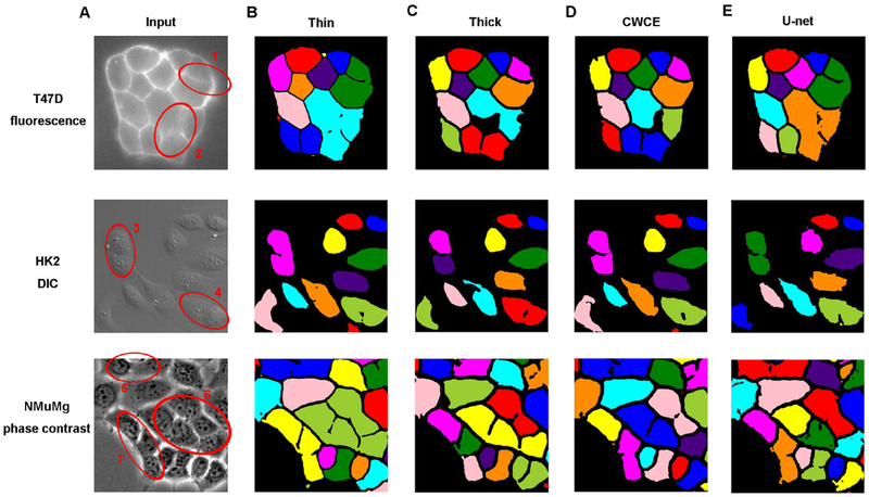
Figure 3.
Example input images and outputs of the pixel-wise classification algorithm.
Red circles highlight cells that have blurry boundaries and are mis-segmented by some or all methods tested here.

Figure 4.
Example output of the combined method applied to different types of images.
The four columns are input images, predicted EDT, cell detection (bounding box) results with faster R-CNN, and watershed segmentation results, respectively.

Figure 5.
Comparison between segmentation accuracy achieved by pixel-wise classification FCNs and the combined method on different types of images.
A: CCA; B: pixel accuracy; C: mean IU.
Figure images are served from the NIH/NLM PubMed Central Open Access Subset or Europe PMC; copyright remains with the publishers and authors.
💬 Discussion
0 commentsNo comments yet. Be the first to start a discussion!
Leave a Comment