Abstract
Machine learning (ML), particularly deep learning (DL), has made rapid and substantial progress in synthetic biology in recent years. Biotechnological applications of biosystems, including pathways, enzymes, and whole cells, are being probed frequently with time. The intricacy and interconnectedness of biosystems make it challenging to design them with the desired properties. ML and DL have a synergy with synthetic biology. Synthetic biology can be employed to produce large data sets for training models (for instance, by utilizing DNA synthesis), and ML/DL models can be employed to inform design (for example, by generating new parts or advising unrivaled experiments to perform). This potential has recently been brought to light by research at the intersection of engineering biology and ML/DL through achievements like the design of novel biological components, best experimental design, automated analysis of microscopy data, protein structure prediction, and biomolecular implementations of ANNs (Artificial Neural Networks). I have divided this review into three sections. In the first section, I describe predictive potential and basics of ML along with myriad applications in synthetic biology, especially in engineering cells, activity of proteins, and metabolic pathways. In the second section, I describe fundamental DL architectures and their applications in synthetic biology. Finally, I describe different challenges causing hurdles in the progress of ML/DL and synthetic biology along with their solutions.
🧬 Organisms
✨ Fluorophores
🧪 Sample Preparation
🔬 Cell Lines
💻 Software Details
🏛️ Research Organizations (ROR)
Affiliated research institutions:
📋 Methods
Categories of Ml Methods
ML is an AI subset that enables computers to acquire knowledge from experience. ML algorithms employ computational approaches to “learn” particulars directly from data without depending on a preordained equation as a representation. The ML algorithms advance their performance adaptively in the presence of excess samples available for learning. In general, the more the training data, the more accurate and precise the learned function. Tens of thousands of ML algorithms exist, and hundreds of new ones are developed annually. When creating an ML model, input representation, loss function, output variables, hyperparameters, and model evaluation are significant considerations. The types of ML are described below in brief. Supervised Machine Learning (SML) SML is the most fundamental type of ML in which an algorithm is instructed on the labeled data. SML methods identify patterns of correlation between input attributes and output variables. The objective is to learn a task that perfectly delineates the relationship between the input attributes and output value in labeled data. Generally, there is direct a relation between the training data and the accuracy of learned tasks, however, the entailed size of training data also relies upon the attributes employed for the specific task. This solution is subsequently deployed for usage with the final data set, from which it learns in the same way as it learned from the training data set. In regression type, an output label is real-valued continuous variables whereas in classification type, the output label is a discrete variable ( Figure 2 A). Figure 2 Schematic representation of machine learning scenarios and mathematical frameworks. (A) SML in which data sets involve ground truth labels. (B) UML in which data sets do not involve ground truth labels. (C) Reinforcement learning where interaction between an algorithmic agent and simulated environment takes place. (D) Linear regression/classification that can be employed to fit models in which the output is a scalar value and data can be predicted by a straight line. (E) Support vector machines locate a separating hyper-plane that parts data into classes. (F) RFs employ the “bagging” technique to construct complete decision trees (DTs) in parallel using random bootstrap instances of the data sets and attributes. RFs select the most labels between different randomized DTs. (G) k-NN is employed for both regression as well as classification, and the input comprises the k nearest training instances in the data set. The output relies on whether the k -NN is employed for regression or classification. (H) NNs generally form a feedforward network of weights in which inputs trigger the hidden layers which give output. However, NNs also form a feedback network in which NNs learn by back-propagation through the networks. Unsupervised Machine Learning (UML) UML has the advantage of working with unlabeled data. The algorithms employ clustering approaches, clustering data points with identical attributes into prominent features with little information loss. Hence, the appraisal generally depends on fact-finding analysis. These algorithms attempt to apply approaches to the input data to explore for rules, find patterns, summarize and cluster data points, derive useful insights, and better communicate the data to users ( Figure 2 B). For more details on SML and UML, I refer the readers to an ML-based book. 17 Reinforcement Learning (RL) RL is directly inspired by how humans learn from events in their daily lives. It has an algorithm that uses trial and error to better itself and learn from new scenarios. Favorable outputs are rewarded, and nonfavorable outputs are rejected. Reinforcement learning, which is built on the psychological idea of conditioning, works by setting the algorithm in a workplace setting with an interpreter and rewards. The output result is delivered to the interpreter at every algorithmic iteration, which decides if the outcome is beneficial or not. If the result is favorable, the interpreter reinforces it by rewarding the algorithm whereas, in case of unfavorable results, the algorithm is compelled to repeat until a better result is found. Generally, the reward system is closely related to the efficacy of the outcome. Due to the availability of large training data sets from simulations under various genetic settings, RL algorithms can provide an efficient computational method to aid in decision-making in the DBTL cycle ( Figure 2 C). Semisupervised Machine Learning (SSML) By employing small labeled and large unlabeled data sets, SSML boosts the efficiency of a supervised model. It can reduce the requirement for vast amounts of organized and human-labeled data along with filtering the systemic noise arising in biological measurements due to various experimental variables. Because SSML is compatible with small training sets, it may have considerable potential in organisms, particularly metazoans with fewer experiment-aided genetic interactive gene pairs. Active Learning (AL) AL is a special case of SML. This method is used to create an effective classifier while minimizing the amount of the training data set by actively organizing the valuable data points. Transfer Learning (TL) Standard ML approaches presume that the training and testing contexts have the same probability distribution. This assumption, however, does not hold in the situation of merging biological data from several platforms. TL refers to the situation when a classifier is trained on one data set and then tested on another data set that may have a completely diverse probability distribution function. Biological data produced from several platforms and maybe employing various technologies is an obvious option for transfer learning approaches. For example, features acquired from the prediction of yeast growth rate may be transferred to other predictive tasks, 18 including predicting ethanol generation in yeast.
Show full methods section
Categories of Ml Methods
ML is an AI subset that enables computers to acquire knowledge from experience. ML algorithms employ computational approaches to “learn” particulars directly from data without depending on a preordained equation as a representation. The ML algorithms advance their performance adaptively in the presence of excess samples available for learning. In general, the more the training data, the more accurate and precise the learned function. Tens of thousands of ML algorithms exist, and hundreds of new ones are developed annually. When creating an ML model, input representation, loss function, output variables, hyperparameters, and model evaluation are significant considerations. The types of ML are described below in brief. Supervised Machine Learning (SML) SML is the most fundamental type of ML in which an algorithm is instructed on the labeled data. SML methods identify patterns of correlation between input attributes and output variables. The objective is to learn a task that perfectly delineates the relationship between the input attributes and output value in labeled data. Generally, there is direct a relation between the training data and the accuracy of learned tasks, however, the entailed size of training data also relies upon the attributes employed for the specific task. This solution is subsequently deployed for usage with the final data set, from which it learns in the same way as it learned from the training data set. In regression type, an output label is real-valued continuous variables whereas in classification type, the output label is a discrete variable ( Figure 2 A). Figure 2 Schematic representation of machine learning scenarios and mathematical frameworks. (A) SML in which data sets involve ground truth labels. (B) UML in which data sets do not involve ground truth labels. (C) Reinforcement learning where interaction between an algorithmic agent and simulated environment takes place. (D) Linear regression/classification that can be employed to fit models in which the output is a scalar value and data can be predicted by a straight line. (E) Support vector machines locate a separating hyper-plane that parts data into classes. (F) RFs employ the “bagging” technique to construct complete decision trees (DTs) in parallel using random bootstrap instances of the data sets and attributes. RFs select the most labels between different randomized DTs. (G) k-NN is employed for both regression as well as classification, and the input comprises the k nearest training instances in the data set. The output relies on whether the k -NN is employed for regression or classification. (H) NNs generally form a feedforward network of weights in which inputs trigger the hidden layers which give output. However, NNs also form a feedback network in which NNs learn by back-propagation through the networks. Unsupervised Machine Learning (UML) UML has the advantage of working with unlabeled data. The algorithms employ clustering approaches, clustering data points with identical attributes into prominent features with little information loss. Hence, the appraisal generally depends on fact-finding analysis. These algorithms attempt to apply approaches to the input data to explore for rules, find patterns, summarize and cluster data points, derive useful insights, and better communicate the data to users ( Figure 2 B). For more details on SML and UML, I refer the readers to an ML-based book. 17 Reinforcement Learning (RL) RL is directly inspired by how humans learn from events in their daily lives. It has an algorithm that uses trial and error to better itself and learn from new scenarios. Favorable outputs are rewarded, and nonfavorable outputs are rejected. Reinforcement learning, which is built on the psychological idea of conditioning, works by setting the algorithm in a workplace setting with an interpreter and rewards. The output result is delivered to the interpreter at every algorithmic iteration, which decides if the outcome is beneficial or not. If the result is favorable, the interpreter reinforces it by rewarding the algorithm whereas, in case of unfavorable results, the algorithm is compelled to repeat until a better result is found. Generally, the reward system is closely related to the efficacy of the outcome. Due to the availability of large training data sets from simulations under various genetic settings, RL algorithms can provide an efficient computational method to aid in decision-making in the DBTL cycle ( Figure 2 C). Semisupervised Machine Learning (SSML) By employing small labeled and large unlabeled data sets, SSML boosts the efficiency of a supervised model. It can reduce the requirement for vast amounts of organized and human-labeled data along with filtering the systemic noise arising in biological measurements due to various experimental variables. Because SSML is compatible with small training sets, it may have considerable potential in organisms, particularly metazoans with fewer experiment-aided genetic interactive gene pairs. Active Learning (AL) AL is a special case of SML. This method is used to create an effective classifier while minimizing the amount of the training data set by actively organizing the valuable data points. Transfer Learning (TL) Standard ML approaches presume that the training and testing contexts have the same probability distribution. This assumption, however, does not hold in the situation of merging biological data from several platforms. TL refers to the situation when a classifier is trained on one data set and then tested on another data set that may have a completely diverse probability distribution function. Biological data produced from several platforms and maybe employing various technologies is an obvious option for transfer learning approaches. For example, features acquired from the prediction of yeast growth rate may be transferred to other predictive tasks, 18 including predicting ethanol generation in yeast.
Optimal Experimental Design
When compared to other domains, data tagging for synthetic biology challenges is frequently quite expensive, requiring professional knowledge of the subject and, in some cases, sophisticated laboratory-based data-gathering systems. This cost is especially problematic for deep learning models requiring outstanding training data. It increases interest in ensuring practitioners do not squander time and resources in classifying data, not adding much to a model. The selection of appropriate data to label or tests to run is an optimum experimental design termed active learning in the ML community. The usage of this method to solve DL problems can greatly minimize data set development costs. 148 , 149 DL algorithms for optimal experimental design are not yet extensively employed in engineering biology; nonetheless, the ability of laboratory automation and initial findings based on simulation indicates that this is a viable area for future research. Treloar et al. 150 employed deep reinforcement learning for controlling a simulated chemostat representation of a microbial coculture developing in a continuous bioreactor. The authors showed that by running five bioreactors in tandem for 24 h a reasonable control policy can be gained and that deep reinforcement learning can be employed to determine the best pattern of inputs and control actions to pertain to a continuous chemostat to increase the product performance of a microbial coculture bioprocess. It is a computational example of a DL-driven optimal experimental design in which reinforcement learning is employed to estimate near-optimal patterns of bioreactor inputs to manage a complicated system ( Figure 8 ). Future work in optimum experimental design can rely on existing ML algorithms, such as those used in metabolic engineering applications. 54 , 63 , 151 − 153 Figure 8 Learning a proposed plan in 24 h. (A) Training of reinforcement learning agent was conducted online for 24 h on a model comprising five parallel chemostats. (B) Shows the reward obtained from the surroundings. Despite a little standard difference in reward, all five chemostats had been relocated to the intended population levels by the completion of the simulation. (C) Exhibit the population curve of one chemostat. The population levels change, and random actions are conducted throughout the exploration phase. When the exploring rate declines, the population levels approach the target values. Reproduced from ref ( 150 ) (an open access article distributed under the terms of the Creative Commons Attribution License). Copyright 2020, Treloar et al.
Latest DL Methods to Address the Challenges and Outlook In this section I have presented the latest DL methods and perspectives for addressing the above-mentioned challenges. Pretrained Self-Supervised Models for Alleviating the Challenge of Data Insufficiency Pretrained models can achieve state-of-the-art performance on various natural language processing (NLP) tasks. Pretrained models like BERT, 174 GPT, 175 − 177 and others are trained on massive corpora of text data. They are exposed to a vast amount of diverse language patterns, which helps them learn rich and contextualized representations of words and sentences. The pretraining process in these models involves self-supervised learning tasks, such as masked language modeling and causal language modeling. These tasks require the model to predict masked or next tokens, forcing it to learn contextual relationships within the text. Pretrained models exhibit strong transfer learning capabilities. They can be fine-tuned on specific downstream tasks with relatively small amounts of labeled data. The pretrained knowledge about language and context, captured during pretraining, acts as a powerful template for these downstream tasks. Pretrained models can be updated and adapted to new data without retraining from scratch. This ability to perform continual learning allows them to stay relevant and adapt to changing data distributions. The pretrained models for processing biological sequences, particularly protein and DNA sequences, are inspired by transformer-based architectures, like BERT, but adapted to handle the unique characteristics of biological data. For instance, Rives et al. 178 developed ESM-1b (Evolutionary Scale Modeling) which is a 33-layer Transformer model with 650 million parameters developed for protein sequence modeling. It is trained using BERT-like masked language modeling on a large data set of 250 million protein patterns from Uniref 50, 179 which contains clusters of patterns with 50% similarity in the UniProt Archive. By fine-tuning small data sets, downstream classifiers achieve strong performance on tasks like predicting protein secondary structure and contact map. DNABERT 180 is developed for DNA sequence modeling and is based on a 12-layer BERT-base 174 Transformer model with 110 million parameters. It is pretrained on the k-mer portrayal of the human genome using masked language modeling, where the human genome is tokenized into k-mers. DNABERT exhibits similar or superior performance compared to other models on various sequence classification tasks, including promoter recognition, functional genetic variant classification, splice site prediction, and TF binding site prediction. Additionally, DNABERT demonstrates cross-species transfer learning capability by predicting mouse TF binding sites. The MSA Transformer 181 (Multiple Sequence Alignment Transformer) extends the transformer model to handle MSAs of amino acid sequences. By leveraging contextual information within individual sequences and across homologous sequences, the MSA Transformer shows even better performance on downstream tasks like protein secondary structure and contact map prediction compared to ESM-1b. Overall, the use of language modeling as a pretraining objective enables pretrained models to efficiently learn from vast amounts of diverse and unlabeled biological sequence data. Language modeling can create context-dependent representations which can be used to improve performance on various biological prediction tasks. For instance, LM of proteins can develop context-dependent representations, and these representations can be employed to improve the performance of several protein prediction tasks. Moreover, with the understanding of protein likelihood, a researcher can filter, autocomplete, and generate new proteins. However, for this goal, language models should be capable of generating high contextual understanding related to protein sequencing from all domains of interest. This approach has significantly advanced the field of bioinformatics and computational biology, providing powerful tools for biological sequence analysis and prediction tasks. Few-Shot or/and Meta-Learning Mechanisms Result in Data Efficient DL Models The challenge of data insufficiency can also be tackled by developing a DL model that uses data efficiently. Meta-learning is useful in scenarios with limited labeled data, few-shot or one-shot learning settings, and tasks with high variability. DeeReCT-TSS 182 is a deep learning model designed for predicting transcription start sites (TSS) in different cell types. The authors applied a gradient-based meta-learning algorithm called Reptile to facilitate fast adaptation of the TSS prediction model to multiple cell types. The use of Reptile allowed the model to quickly adapt to new cell types with minimal labeled data from each cell type. Mutual information maximization meta-learning (MIMML) 183 is a novel meta-learning framework designed specifically for predicting the function of bioactive peptide. It leverages the Prototypical Network, which is a few-shot learning approach used for classification tasks, to perform predictions for a total of 16 different peptide functions. Benefit Modeling by Including Structural Information The sequence-only models are limited to explicitly consider transacting factors. Such factors usually depend on protein–protein 184 − 187 and protein–nucleic acid interactions at a molecular level. Hence, to accurately model these factors in gene regulation, it is essential to incorporate structural information from both cis-acting and trans-acting counterparts. Indeed, recent breakthroughs in protein structure prediction, particularly the development of AlphaFold2, have significantly advanced our understanding of protein structures. 188 AlphaFold2, developed by DeepMind, demonstrated remarkable accuracy in predicting protein 3D structures during the Critical Assessment of Structure Prediction (CASP) competition. This breakthrough has enriched our resource for protein structures and has the potential to transform the field of structural biology. Additionally, progress has been made in predicting secondary structures of RNA and 3D structures of the genome. 189 − 192 The availability of accurate structural information for proteins, the genome, and RNA opens new possibilities for systematically incorporating this structural information into deep-learning models for gene regulation. By integrating structural data with deep-learning approaches, researchers can create more comprehensive and precise models of gene regulation at the molecular level. Incorporating structural information from protein 3D structures into DL models has the potential to enhance our understanding of complex biological processes and regulatory networks. By leveraging the insights gained from MaSIF 193 and dMaSIF, 194 researchers can explore new avenues for modeling gene regulation, protein–protein interactions, protein–ligand interactions, and other molecular interactions, ultimately leading to advancements in proteomics and systems biology. Indeed, NucleicNet 195 is an excellent example of a transcriptomic-level model that incorporates structural information to predict binding specificities of RNA-binding proteins (RBPs). By representing the binding 3-D structure of protein as a 3-D grid with physicochemical possessions and using a CNN with residual connections, NucleicNet achieves accurate predictions of RBP binding preferences for different RNA constituents. Multiomic Model Development Indeed, biologists often employ multiple experimental techniques to strengthen the validity and reliability of their findings. By using different methods, they can cross-validate their results and reduce the likelihood of errors or biases. The work by Chaudhary et al. 196 is an excellent example of utilizing multiomics data and DL techniques for the prediction of survival of patients with hepatocellular carcinoma (HCC). The model was trained employing 230 samples from TCGA (The Cancer Genome Atlas) with RNA-seq data, DNA methylation profiles, and microRNA-seq data. The process of autoencoder-based dimensionality reduction, 197 feature selection, and concatenation helps to mitigate the challenges posed by high-dimensional omics data and enhances the model’s ability to capture relevant biological signals. The integration of multiomics data with concepts from multimodal machine learning 198 holds great potential for driving innovations in precision medicine and personalized healthcare. The MOMA 199 (Multi-Omics Model and Analytics) model is a sophisticated approach used to predict multiomics quantities of E . coli based on different growth conditions. MOMA combines RNN-based DL and LASSO (Least Absolute Shrinkage and Selection Operator) regression to achieve its predictions. The model acquires a layer-by-layer process to predict proteomic, transcriptomic, metabolomic, phenomic, and fluxomic quantities sequentially, while considering the influence of quantities from previous omics layers on the current prediction. The Deep Structured Phenotype Network (DSPN) 200 is a powerful model designed to predict brain phenotypes using several functional genomic data modalities. The DSPN utilizes a hierarchical conditional deep Boltzmann machine (DBM) architecture 201 for its predictions. This approach allows the model to capture complex interactions and dependencies between different genomic data types and their relationships to brain phenotypes. Usage of Single-Cell Profiles The advanced single-cell omics technologies have greatly expanded our understanding of cellular diversity, developmental processes, disease mechanisms, and the complexity of various tissues and organs. They continue to be refined and applied in diverse fields, from developmental biology and immunology to cancer research and regenerative medicine. Single-cell ATAC-seq (scATAC-seq) 202 , 203 for chromatin accessibility profiling, single-cell RNA-seq (scRNA-seq) for gene expression level profiling, single-cell reduced representation bisulfite sequencing (scRRBS-seq) 204 for methylation profiling, single-cell bisulfite sequencing (scBS-seq), 205 Smartseq 206 for full-length transcriptome profiling, and single-cell Ch IP-seq (scChIP-seq) 207 for protein–DNA binding profiling are some of the key single-cell omics profiling technologies that have seen substantial improvements. Current DL-based gene regulation models use single-cell profiles basically in two different ways. One operates at the genuine single-cell level, while the other operates at the pseudobulk level. Current DL-based gene regulation architectures generally employ single-cell profiles in two divergent ways. The first works at the pseudobulk level. The model assembles single-cell assessments of each cell cluster into a single profile. The assembled pseudobulk profiles are then used by the model in a manner like how bulk omics profiles are used. Regardless of loss of information during aggregation, the employment of pseudobulk profiles still has an advantage over real bulk omics profiles as they depict evaluations from pure cell types without interference from others. The utilization of pseudobulk profiles in the context of single-cell omics analysis has advantages over real bulk omics profiles, despite the information loss that occurs during the aggregation process. The study conducted by Cusanovich et al. 208 involved single-cell ATAC sequencing (scATAC-seq) on around 100,000 somatic cells of mature mice. The researchers aimed to predict chromatin accessibility for each identified cell type using a multitask learning approach based on the Basset architecture. They trained the model based on aggregated pseudobulk profiles inside each cell cluster. Recently, based on DeepMEL, Janssens et al. presented DeepFlyBrain model for predicting chromatin coaccessible areas in the Drosophila brain. 209 DeepCpG 210 is a deep learning model designed for imputing methylation status in low-coverage single-cell DNA methylation profiles. The model was trained on scBS-seq (single-cell bisulfite sequencing) and scRRBS-seq (single-cell reduced representation bisulfite sequencing) data from multiple mouse and human tissues. The model architecture combines CNNs with bidirectional Gated Recurrent Units (GRUs). SCALE 211 is a DL model designed for imputing low-coverage single-cell ATAC sequencing (scATAC-seq) profiles. The model is based on a combination of variational autoencoder (VAE) and Gaussian mixture models (GMMs). It is specifically tailored to address the challenge of handling sparse and missing data in scATAC-seq profiles. DL approaches have also shown promising results in making inferences on gene regulation networks employing single-cell RNA seque (scRNA-seq) data. CNNC 212 is one such example of a DL model designed for inferring the causality between two genes in a gene regulatory network. Many latest methods and perspectives to overcome the challenges have been summarized in table format 213 − 245 ( Table S1 ).
Supplementary Material ao3c05913_si_001.pdf
📊 Figures
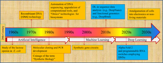
Figure 1
An overview of the advancesnin ML/DL and synthetic biology sincenthe 1960s.
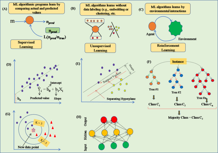
Figure 2
Schematic representation of machine learningnscenarios and mathematicalnframeworks. (A) SML in which data sets involve ground truth labels.n(B) UML in which data sets do not involve ground truth label...
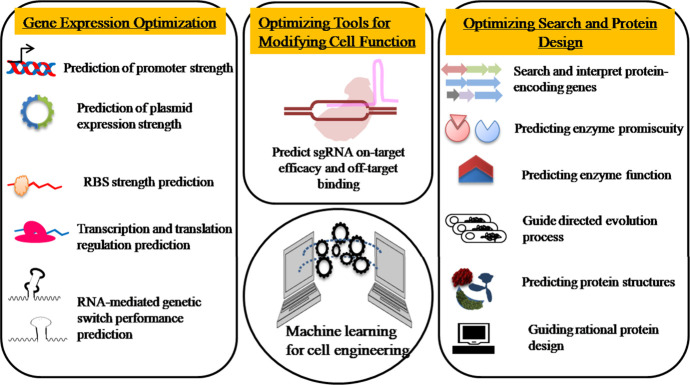
Figure 3
Applications of ML in cell engineering. ML can be employed forn(i) improving gene expression, (ii) bettering tools for altering cellularnfunctions, and (iii) upgrading protein search and design.
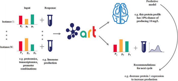
Figure 4
ART gives predictions and recommendations for the followingncycle.nART employs experimental data for (i) constructing a probable predictivenrepresentation that predicts response from input variables a...
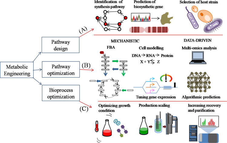
Figure 5
Applications of ML in metabolic engineering systems. Inngeneral,na metabolic engineering venture can be divided into three parts: (i)nmetabolic pathway design, (ii) boosting cells for production, andn...
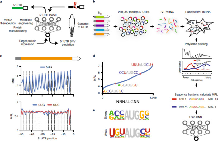
Figure 6
Library consistsnof 280,000 random 50 nucleotide oligomers as 5u2032nuntranslated regions (UTRs) for enhanced green fluorescent proteinn(eGFP). (A) Shows the usage of a 5u2032 UTR to assess the potent...
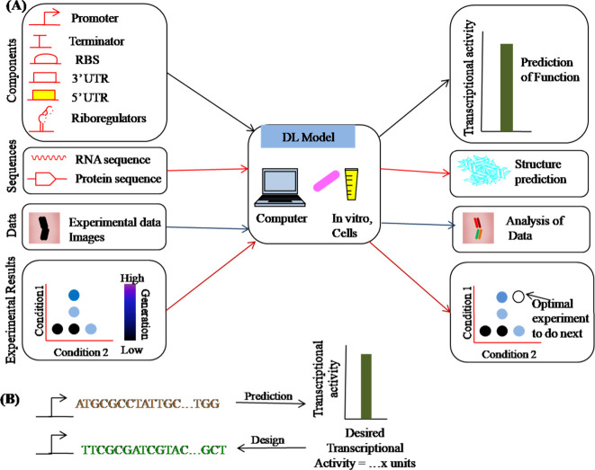
Figure 7
DL enabled applicationsnof synthetic biology. (A) Representativencases of pertinent inputs to DL networks and their allied output predictions.n(B) Given a fresh input, predictions can be made using de...
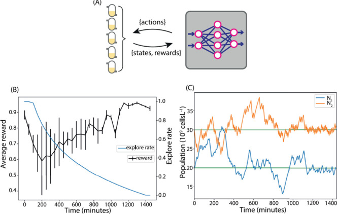
Figure 8
Learning a proposed plan in 24 h. (A) Trainingnof reinforcementnlearning agent was conducted online for 24 h on a model comprisingnfive parallel chemostats. (B) Shows the reward obtained from the surr...
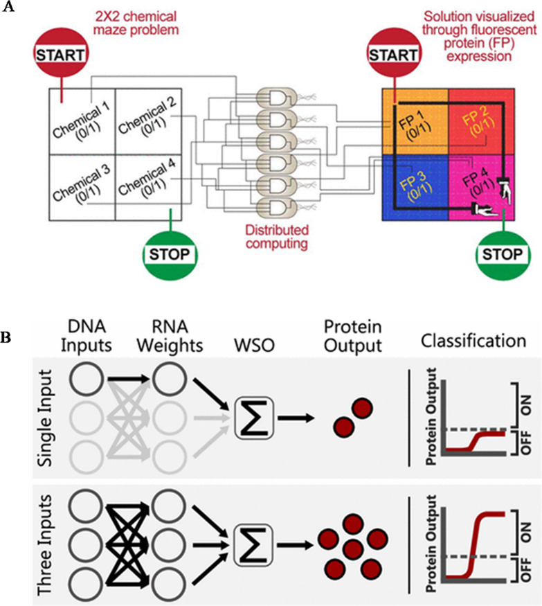
Figure 9
(A) Application of thendistribution of simple genetic circuitsnamong bacterial populations to solve chemically produced 2 u00d7n2 maze issues by selectively articulating four distinct fluorescentnprot...
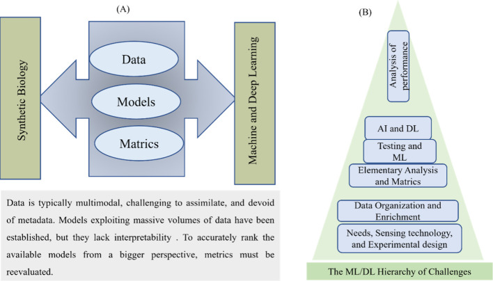
Figure 10
(A) Challenges of amalgamating ML/DL techniquesnwith applicationsnof synthetic biology. (B) A standard ML/DL framework can help syntheticnbiology research. The intermediate stages are typically the ce...
Figure images are served from the NIH/NLM PubMed Central Open Access Subset or Europe PMC; copyright remains with the publishers and authors.
💬 Discussion
0 commentsNo comments yet. Be the first to start a discussion!
Leave a Comment