Abstract
Neural activation increases blood flow locally. This vascular signal is used by functional imaging techniques to infer the location and strength of neural activity. However, the precise spatial scale over which neural and vascular signals are correlated is unknown. Furthermore, the relative role of synaptic and spiking activity in driving haemodynamic signals is controversial. Previous studies recorded local field potentials as a measure of synaptic activity together with spiking activity and low-resolution haemodynamic imaging. Here we used two-photon microscopy to measure sensory-evoked responses of individual blood vessels (dilation, blood velocity) while imaging synaptic and spiking activity in the surrounding tissue using fluorescent glutamate and calcium sensors. In cat primary visual cortex, where neurons are clustered by their preference for stimulus orientation, we discovered new maps for excitatory synaptic activity, which were organized similarly to those for spiking activity but were less selective for stimulus orientation and direction. We generated tuning curves for individual vessel responses for the first time and found that parenchymal vessels in cortical layer 2/3 were orientation selective. Neighbouring penetrating arterioles had different orientation preferences. Pial surface arteries in cats, as well as surface arteries and penetrating arterioles in rat visual cortex (where orientation maps do not exist), responded to visual stimuli but had no orientation selectivity. We integrated synaptic or spiking responses around individual parenchymal vessels in cats and established that the vascular and neural responses had the same orientation preference. However, synaptic and spiking responses were more selective than vascular responses--vessels frequently responded robustly to stimuli that evoked little to no neural activity in the surrounding tissue. Thus, local neural and haemodynamic signals were partly decoupled. Together, these results indicate that intrinsic cortical properties, such as propagation of vascular dilation between neighbouring columns, need to be accounted for when decoding haemodynamic signals.
🔬 Techniques
🔭 Microscopes
💻 Software
✨ Fluorophores
🧪 Sample Preparation
🔬 Cell Lines
🏭 Microscope Brands
🧪 Reagent Suppliers
🔴 Lasers
💻 Software Details
💾 Data Repositories
🏛️ Research Organizations (ROR)
Affiliated research institutions:
📋 Methods
Animals and surgery
All surgical and experimental procedures were approved by the Institutional Animal Care and Use Committee at Medical University of South Carolina. Cats ( n = 25 of either sex; postnatal day 28 to > 2.5 kg adult) were anesthetized with isoflurane (1–2% during surgery, 0.5–1.0% during imaging) and paralyzed with a continuous infusion of vecuronium bromide (0.2 mg kg -1 hr -1 , intravenously). Cats were artificially ventilated through a tracheal cannula, and the end tidal CO 2 was regulated at 3.5–4.5%. Heart rate, respiration rate, temperature and electroencephalogram were also monitored. Long Evans rats ( n = 10 males, postnatal days 31–45) and C57Bl/6J mice ( n = 1 male, postnatal day 63) were initially anaesthetized with a bolus infusion of fentanyl citrate (0.04–0.06 mg kg -1 ), midazolam (3.75–6.25 mg kg -1 ), and dexmedetomidine (0.19–0.31 mg kg -1 ). The one mouse was used for a control experiment to confirm that the iGluSnFR sensor was not being saturated during sensory stimulation (see Methods below). During two-photon imaging, continuous intraperitoneal infusion with a lower concentration mixture (fentanyl citrate: 0.02–0.03 mg kg -1 h -1 , midazolam: 1.50–2.50 mg kg -1 h -1 , and dexmedetomidine: 0.10–0.25 mg kg -1 h -1 ) was administered using a catheter connected to a syringe pump. For all animals, craniotomies (2–3 mm square) were opened over the primary visual cortex (area 18), the dura was reflected, and the craniotomies were sealed with agarose (1.5–3% dissolved in artificial cerebrospinal fluid ACSF) and a glass coverslip. When the calcium indicator Oregon Green 488 Bapta-1 AM (OGB-1 AM) was used, prior to the placement of the coverglass, a pipette was inserted into the craniotomy and the dye was injected with air pressure puffs. The dye loading procedure has been described in detail 31 . In cats, we also used the genetically encoded indicators GCaMP6s 32 and iGluSnFR 33 to measure calcium and glutamate activity respectively. Two to four weeks prior to the imaging session, viral injections of AAV2/9.hSyn.GCaMP6s.WPRE.SV40 or AAV2/1.hSyn.iGluSnFR.WPRE.SV40 were performed under sterile surgery conditions. Cats were anesthetized with 1–2% isoflurane and vital signs were monitored. One to three craniotomies were performed over the primary visual cortex (area 18) and small holes were made in the dura. Aliquots of virus (5 μL) were diluted in phosphate buffer saline (PBS) and mannitol (5:9:6 ratio of virus:PBS:mannitol) to titers of ∼10 12 genomes ml -1 with 50–200 nL of Fast Green dye (Sigma) added to visualize the injection. Glass pipettes containing the virus solution were lowered 500–800 μm into the cortex and pressure puffs were administered over 15–20 minutes until approximately 1 μL had been injected. After 10 minutes, the pipettes were slowly retracted, the craniotomies were sealed with agarose (3% dissolved in ACSF), the scalp was sutured closed and the animals were recovered and returned to their housing. All animals were treated similarly and so randomization and blinding were not required. No statistical methods were used to predetermine sample size.
Show full methods section
Animals and surgery
All surgical and experimental procedures were approved by the Institutional Animal Care and Use Committee at Medical University of South Carolina. Cats ( n = 25 of either sex; postnatal day 28 to > 2.5 kg adult) were anesthetized with isoflurane (1–2% during surgery, 0.5–1.0% during imaging) and paralyzed with a continuous infusion of vecuronium bromide (0.2 mg kg -1 hr -1 , intravenously). Cats were artificially ventilated through a tracheal cannula, and the end tidal CO 2 was regulated at 3.5–4.5%. Heart rate, respiration rate, temperature and electroencephalogram were also monitored. Long Evans rats ( n = 10 males, postnatal days 31–45) and C57Bl/6J mice ( n = 1 male, postnatal day 63) were initially anaesthetized with a bolus infusion of fentanyl citrate (0.04–0.06 mg kg -1 ), midazolam (3.75–6.25 mg kg -1 ), and dexmedetomidine (0.19–0.31 mg kg -1 ). The one mouse was used for a control experiment to confirm that the iGluSnFR sensor was not being saturated during sensory stimulation (see Methods below). During two-photon imaging, continuous intraperitoneal infusion with a lower concentration mixture (fentanyl citrate: 0.02–0.03 mg kg -1 h -1 , midazolam: 1.50–2.50 mg kg -1 h -1 , and dexmedetomidine: 0.10–0.25 mg kg -1 h -1 ) was administered using a catheter connected to a syringe pump. For all animals, craniotomies (2–3 mm square) were opened over the primary visual cortex (area 18), the dura was reflected, and the craniotomies were sealed with agarose (1.5–3% dissolved in artificial cerebrospinal fluid ACSF) and a glass coverslip. When the calcium indicator Oregon Green 488 Bapta-1 AM (OGB-1 AM) was used, prior to the placement of the coverglass, a pipette was inserted into the craniotomy and the dye was injected with air pressure puffs. The dye loading procedure has been described in detail 31 . In cats, we also used the genetically encoded indicators GCaMP6s 32 and iGluSnFR 33 to measure calcium and glutamate activity respectively. Two to four weeks prior to the imaging session, viral injections of AAV2/9.hSyn.GCaMP6s.WPRE.SV40 or AAV2/1.hSyn.iGluSnFR.WPRE.SV40 were performed under sterile surgery conditions. Cats were anesthetized with 1–2% isoflurane and vital signs were monitored. One to three craniotomies were performed over the primary visual cortex (area 18) and small holes were made in the dura. Aliquots of virus (5 μL) were diluted in phosphate buffer saline (PBS) and mannitol (5:9:6 ratio of virus:PBS:mannitol) to titers of ∼10 12 genomes ml -1 with 50–200 nL of Fast Green dye (Sigma) added to visualize the injection. Glass pipettes containing the virus solution were lowered 500–800 μm into the cortex and pressure puffs were administered over 15–20 minutes until approximately 1 μL had been injected. After 10 minutes, the pipettes were slowly retracted, the craniotomies were sealed with agarose (3% dissolved in ACSF), the scalp was sutured closed and the animals were recovered and returned to their housing. All animals were treated similarly and so randomization and blinding were not required. No statistical methods were used to predetermine sample size.
Two-photon imaging
For vascular imaging, three fluorescent dyes were used as we described previously 12 . Alexa 633 fluor hydrazide selectively labels artery walls while Texas Red dextran (70 kDa) and fluorescein dextran (2,000 kDa) indiscriminately label the entire vascular lumen. Fluorescein dextran has similar excitation and emission properties as our neuronal labels OGB-1 AM, GCaMP6s, and iGluSnFR. Therefore, fluorescein dextran was not used for vessel dilation measurements in animals where neuronal imaging was performed because sufficient contrast between a vessel wall and background is more difficult to obtain when two green labels are used simultaneously. Fluorescein dextran was typically used for the measurement of RBC velocity and was only injected after the neural imaging was completed. Fluorescence was monitored with a custom-built microscope (Prairie Technologies) coupled with a Mai Tai (Newport Spectra-Physics) mode-locked Ti:sapphire laser (810 nm or 920 nm) with DeepSee dispersion compensation. Excitation light was focused by a 40× (NA 0.8, Olympus), 20× (NA 1.0, Olympus) or 16× (NA 0.8, Nikon) water immersion objective and beam expansion optics. Full frame imaging of neural activity and vessel dilation were typically obtained at approximately 0.8 Hz. All the blood velocity data and the dilation of a small number of vessels were measured with line scans rather than full frame imaging by using line acquisition rates between 0.4 and 4.2 kHz. Visual stimulation and size of imaged region Drifting square-wave grating stimuli were presented on a 17-inch LCD monitor. The gratings were presented at 100% contrast, 30 cd m -2 mean luminance, 1.5–2.0 Hz temporal frequency. As depicted in the various time courses, e.g., Fig. 1 , these stimuli were presented at eight directions of motion in 45° steps and each of these eight stimuli was interspersed with blank periods (equiluminant gray screen). Because vascular responses decay slowly, we used long blank periods (at least 4 times the stimulus duration) when measuring blood vessel responses. We also presented the eight visual stimuli in pseudo-random order. These steps ensured that a particular response would not be influenced by a residual response to the previous stimulus. The duration of the stimulation period, e.g., 6 s, and the duration of the blank period, e.g., 24 s, was always identical across all epochs in a stimulus sequence. Each of the eight stimuli was repeated at least three times and in the vast majority of the data, 5–10 trials were used. Unlike arteriole dilation, neural transients return to baseline nearly immediately upon extinguishing the visual stimulus 12 , 34 (also see Extended Data Figs. 1 and 2 ). Therefore, for epochs of data collection involving only calcium or glutamate imaging, either sequential or pseudo-random sequences were used. While some neural and vascular data were collected simultaneously, our analyses benefited from collecting them sequentially for the following reasons. Neural data was typically collected in 600 × 600 μm square regions to allow the pooling of large regions of activity (see Figs. 2b,c and 3b ) and multiple 600 × 600 μm square regions were often imaged in a single craniotomy to obtain maps where many orientation and direction domains were represented (see Figs. 2b,c , 3b and Extended Data Fig. 1 ). Higher pixel resolution was needed for resolving blood vessel dilation so we usually obtained the vessel responses immediately after the neural responses using higher optical zooms that were centered on the blood vessels of interest. Because of the optical zoom customization per imaged site and the differences in recovery of neural vs. vascular responses to baseline, the selected duration of visual stimulation for a particular experiment ranged from 2–8 s and the duration of blank periods ranged from 6–35 s.
Data-analysis overview
Images were analyzed in Matlab (Mathworks) and ImageJ (National Institutes of Health). Data with significant movements (several μm) in XY or Z were excluded. Data with small drift movements were realigned by maximizing the correlation between frames. Quantifying vessel dilation We analyzed dilation responses only in surface arteries and penetrating arterioles because veins and capillaries do not typically dilate to sensory stimuli less than 10 seconds in duration 12 - 14 . When veins dilate in response to very long duration sensory stimuli, these responses are relatively weak and extremely slow unlike the rapid and large responses of arteries and arterioles 13 . Surface arteries and penetrating arterioles are distinguished from veins using Alexa-633 as an artery specific dye, by their orange vs. purplish hue under bright-field illumination, and by the tone of the vessel walls and the speed and direction of blood flow during two-photon imaging 12 . Distinguishing capillaries from pre-capillary arterioles has been inconsistent in the literature 13 , 14 , 18 , 19 . Here we categorize capillaries as vessels with 4-7 μm baseline diameter 21 , high tortuosity and complete lack of Alexa-633 labeling 12 . Vessel diameter was determined in full-frame images by one of two methods. When the vessel had a circular profile (as was the case for most of the parenchymal arterioles), a region of interest was manually drawn around each vessel and a circle was fit to the pixels in the region that passed a luminance threshold ( Extended Data Fig. 6 ). For vessels with an elongated profile (typical for pial surface vessels), a cross-section was taken through the vessel walls and the peaks in luminance (for the wall-labeling Alexa 633) or peaks in the pixel-by-pixel luminance difference along the line (for lumen labels) were used to compute the diameter 12 (see Extended Data Fig. 7 ). For the few instances where diameter was measured using line-scans, we averaged the data along the time axis over all the lines in an image (usually 1000 lines) or obtained two data points per image by sequentially averaging half the lines in each image. Since each line was only 0.25–2.5 ms in duration, averaging across these lines still provided sufficient temporal resolution for capturing the onset, peak and recovery of sensory-evoked dilation. The diameter was computed from these line scans in the same way as for the cross-section ( Extended Data Fig. 8 ). For all methods of dilation measurement, images were usually oversampled by interpolating between pixels from 2-20 times to allow the algorithm to compute diameter values with a spatial resolution that was finer than the pixel size in the raw data images. To compute the vascular response to each condition, a stimulus response window was defined. Because of the slow onset and offset of the vascular response, we could not simply assign the response period to correspond to the period when the stimulus was displayed on the monitor. Instead, for each vessel we selected the response period by examining the average response across all stimulus conditions and then selected the imaging frames that best approximated this response interval. Shifting this time window by adding or removing data points did not appreciably change the responses. The mean response across this time window was divided by the baseline level for each condition to get the percent-change in diameter. Responsive vessels were defined by ANOVA across baseline and 8 directions over multiple trials ( P < 0.05). The Orientation Selectivity Index (OSI) was defined as: OSI = abs (Σ r k eˆ(i2θ k ) /Σ r k ), where θ k is the orientation of each stimulus and r k is the mean response across trials to that stimulus 35 . Note that OSI = 1 – circular variance. The preferred orientation was defined as: arctan(Σ r k cos(2θ k ) /Σ r k sin(2θ k ) ). The Directionality Index (DI) was computed as 1 – r null /r pref , where r pref is the response amplitude to the preferred stimulus and r null is the response to the stimulus with the same orientation drifting in the opposite direction. Computing the OSI based on flow rather than diameter by scaling the diameter values to the 4 th power (Poiseuille's law) did not affect our results. Measuring onset latency to dilation To compare the latencies of pial arteries and parenchymal arterioles, we fit a linear regression line to the rising phase of the dilation (20-80% of the peak response) of each vessel. For parenchymal vessels, we used only the response to the preferred orientation because of potential latency differences between dilation to the preferred and other stimulus orientations (see below). For the pial vessels, we pooled the response to all stimulus conditions because these vessels are untuned to stimulus orientation. We used the time at which the regression line crossed the pre-stimulus baseline level as the onset latency 12 . This regression line metric on the average response is applicable when responses are large and relatively stable from trial to trial—as is the case for pial vessels to any stimulus orientation and for parenchymal vessels to the preferred stimulus orientation. Since parenchymal vessels are orientation selective ( Fig. 1b,d ), responses to the null orientation are the weakest and, by definition, smallest in amplitude and more noisy from trial to trial. Thus, to compare the latency between the response to the preferred and null orientations in parenchymal vessels, we used a statistical test, the standardized mean difference (SMD, specifically Hedge's g 36 , 37 ), in which vessels are weighted by the trial-by-trial variance in latency values (see Extended Data Fig. 5a ). We first smoothed each trial's time course with a 3 frame running average. We then performed linear regression on the same interval as above (20-80% of the peak). We took the difference in the average onset latency across trials between the responses to preferred and null stimuli and standardized this difference by the pooled variability across the two conditions. The population summary SMD was obtained by using a random-effect model. This model weighs each vessel by the inverse variance of its SMD and factors in the heterogeneity present across the individual vessel data 37 . As a control for spurious effects, the preferred and null responses were assigned randomly for each trial and the analysis was repeated ( Extended Data Fig. 5b ). Quantifying blood velocity Velocity data was analyzed as described previously 22 . Briefly, line scans were first pooled into blocks of 250, 500, or 1000 lines. The angle of the RBC streaks in each image was used to determine the velocity of that block and a time course of velocity measurements was extracted. Baseline and stimulus windows were defined similarly to the dilation data and equivalent OSI and statistical analyses were performed.
Analysis of calcium and glutamate responses
Calcium and glutamate signals were analyzed the same way. Raw images were first smoothed with a 4 μm Gaussian filter. The mean fluorescence of each pixel within a given 100–600 μm-diameter window around a vessel was computed for each blank and stimulus epoch. A t -test was performed on the difference in stimulus and baseline fluorescence for each condition in each trial and if the distribution was significantly higher than zero ( P < 0.05), the pixel was included in the integration window. We also performed this analysis without excluding the unresponsive pixels and the responses were indistinguishable. In some datasets, part of the 100–600 μm diameter analysis window fell outside of the image boundary and so there would be fewer pixels from those domains contributing to the overall response. Therefore, to avoid biasing the overall response of the integrated region, we divided the 100–600 μm diameter analysis window into wedges before averaging the data over the full window. Each wedge was 1/16 of the circle and was further divided into sections of 50 μm radial length. Thus, a 100-μm-diameter window had 16 sections whereas a 400-μm-diameter window had 64. The pixels with significant responses within each section were averaged together to create a time course. The time course was then normalized by a sliding baseline of the mean fluorescence of each blank interval (ΔF/F). Each time course was then weighted by the total number of pixels represented by its section, because sections farther from the vessel contain more pixels. Finally, the time courses of all the sections were averaged together to obtain the time course of the entire region. For inclusion in the population dataset, responses from the 100–600 μm diameter analysis windows had to pass the following criteria. First, each wedge had to have at least 30% of the imaged pixels passing the initial t -test to ensure that windows with wedges having no response and/or weak labeling would be removed. Secondly, at least 80% of the circular area of the window had to be within the image to ensure that a sizeable region of tissue whose orientation preference could dramatically affect the overall response was not being missed. In addition, at least 10% of each wedge had to be within the image to ensure that each wedge had some representation. For data that passed all these criteria, the responses to each condition were computed by averaging the imaging frames during stimulus presentation and across trials. Before the OSI was computed, if any conditions showed a negative response (below the baseline level), then the absolute value of the minimum response was added to all responses (to make the minimum equal zero). We have recently published a mechanistic rationale for applying such a correction in fluorescence imaging of neural responses—stimulus-evoked dilation of surface arteries can block fluorescence from the underlying tissue and make a very small response actually appear negative 12 . We also analyzed the data without this correction and in addition, when only including the first one-second of the response (to avoid the slower surface artery interference 12 ). Although there were small changes in the OSI values of individual windows, the overall results did not change in either case. The neural response amplitudes, OSI and DI were all computed using the same formulae as for the vessel data. Population distribution statistics on OSI and DI measurements used the Mann-Whitney test.
Additional control for calcium imaging
Spiking activity in the neuropil should also contribute to metabolic needs and hence neurovascular coupling. Therefore, when integrating the calcium signals in the tissue surrounding each artery, we included all pixels that passed a signal-to-noise criterion (see previous section) and not only those corresponding to cell bodies. However, the neuropil may include a mixture of calcium signals from synaptic events in dendritic spines and spiking in axons arriving from regions outside of the integration window we selected. Therefore, as a control, we compared the orientation selectivity in 400-μm-diameter windows with and without including the neuropil. Masks excluding the neuropil were generated in the same way as described above except that the pixels within each wedge were constrained to the cell bodies. Cell body masks were first created using an automated algorithm that applied a series of morphological filters to identify the contours of cell bodies based on intensity, size and shape 10 . Cell outlines were visually inspected and errors were corrected manually. Then a t -test was performed on each pixel of these masks and the wedges were created in the same manner as before. Because of the sparse distribution of cell bodies, we did not enforce the 30% significantly responding imaged pixels criterion but all other criteria applied. The orientation selectivity with the two mask types was indistinguishable ( Extended Data Fig. 9 ). Control to show that visual stimulation was not saturating the iGluSnFR sensor With visual stimulation, the glutamate signals peaked at < 10% ΔF/F. To determine if the iGluSnFR sensor responded linearly and responded over a greater range than that obtained with visual stimulation, we used iontophoresis to apply large doses of exogenous glutamate. We lowered a pipette containing 0.5 M glutamate into layer 2/3 of the visual cortex of a mouse that was labelled with iGluSnFR. We applied a range of currents (10, 20, 40, 60, 80 nA) and found that the fluorescence signals increased linearly ( R > 0.99; P < 0.0001) and peaked at ∼ 60% ΔF/F (data not shown). Thus, our in vivo imaging with iGluSnFR (e.g., Extended Data Fig. 10 ) is likely revealing the true spatial profile of glutamate direction maps ( Fig 3 ) and orientation maps ( Extended Data Figure 1 ).
Supplementary Material supp_info
📊 Figures
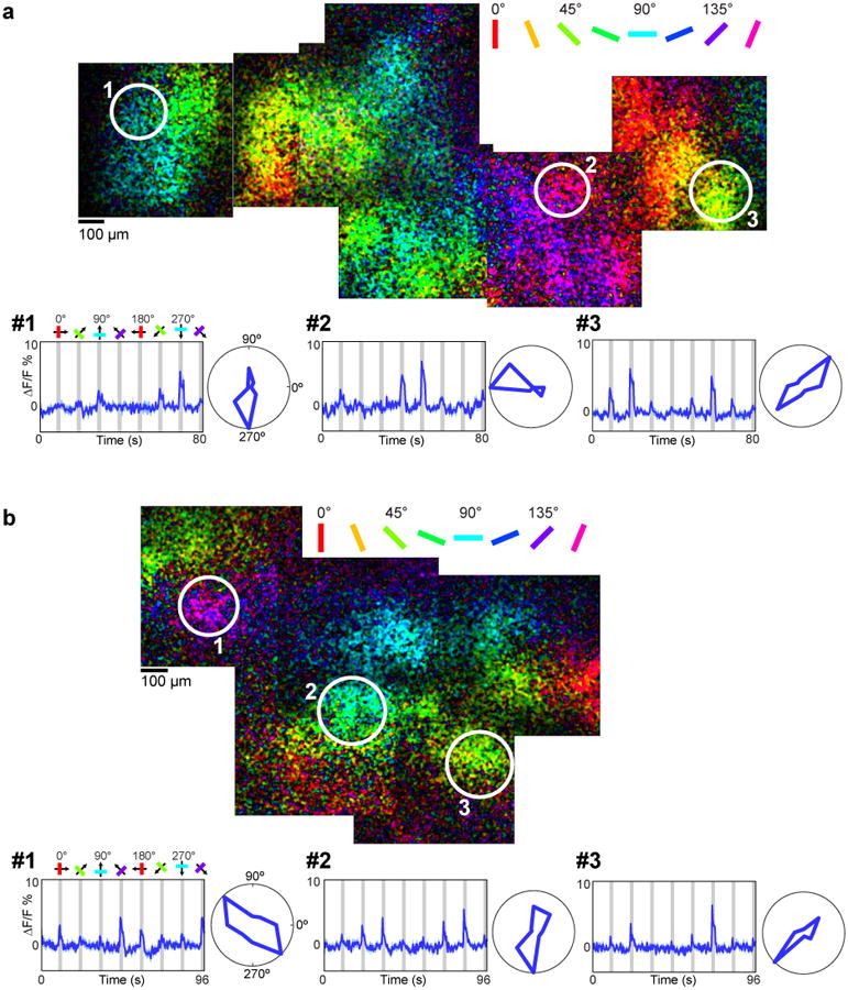
Extended Data Figure 1
Glutamate release is organized into orientation maps
a, Region of cat visual cortex labeled with iGluSnFR. Pixels are color-coded by preferred orientation with the brightness indicating the response strength. Time courses and polar plots (averages of fo...
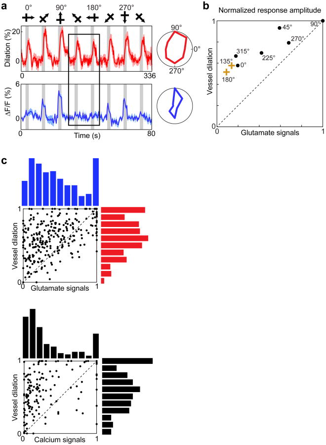
Extended Data Figure 2
Arteriole dilation in the absence of glutamate signaling or local spiking
a, Time courses and polar plots of arteriole dilation (red) and the release of glutamate in a 400-u03bcm-diameter window surrounding an arteriole (blue). Averages of eight trials are shown for vessel ...
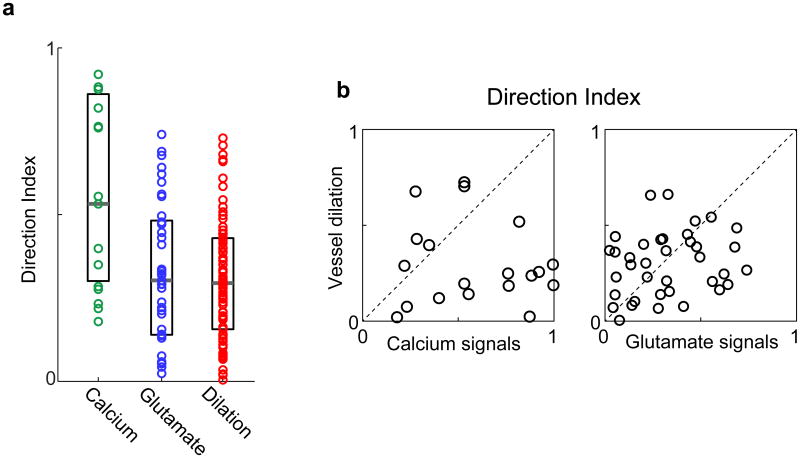
Extended Data Figure 3
Direction selectivity of parenchymal vessels and of local spiking and synaptic activity
a, Population distributions of the direction index of calcium (green, n = 19 windows in 8 cats), glutamate (blue, n = 37 windows in 5 cats) and vessel dilation (red, n = 79 vessels in 18 cats) respons...
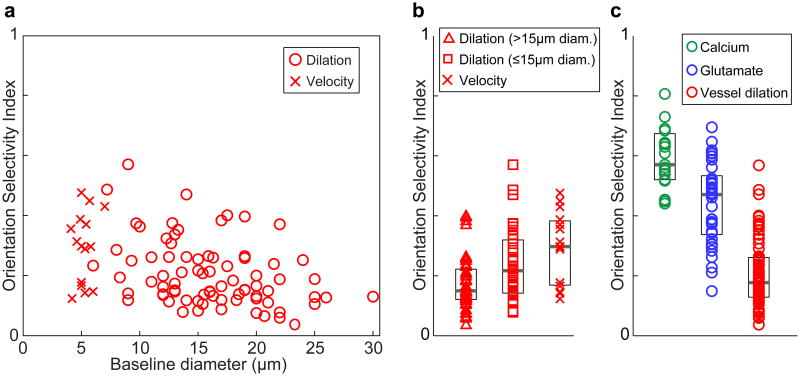
Extended Data Figure 4
Dilation and velocity responses in parenchymal blood vessels with different baseline diameters
a, The diameter of all vessels and their OSI values from cat visual cortex layer 2/3. For arterioles, OSI was determined based on dilation ( n = 79 vessels in 18 cats) whereas for capillaries, OSI was...
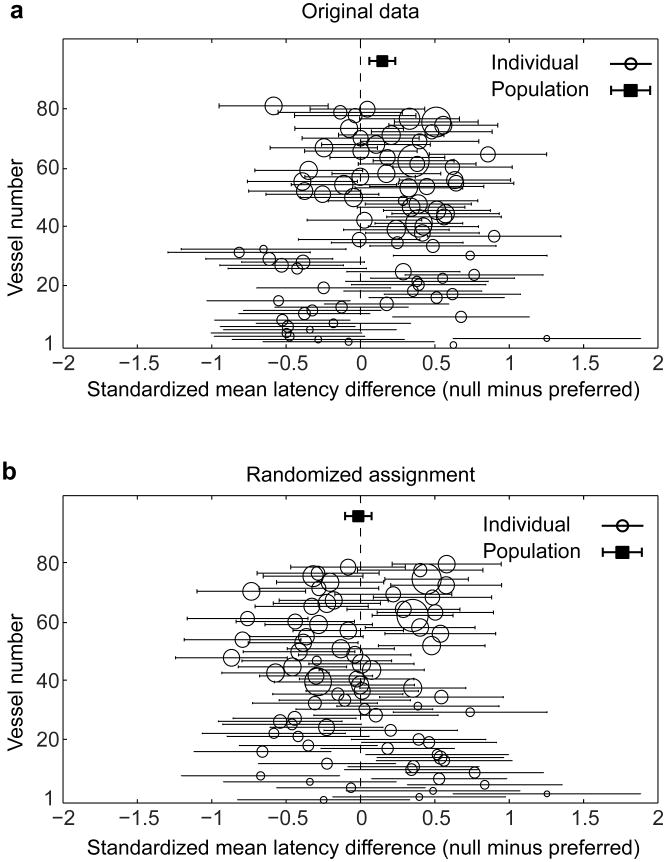
Extended Data Figure 5
Onset latency of dilation in parenchymal vessels
a, Vessel-by-vessel comparison of the onset latency difference between the response to preferred and orthogonal (null) stimulus orientations. Each whisker diagram represents a single vessel with the c...
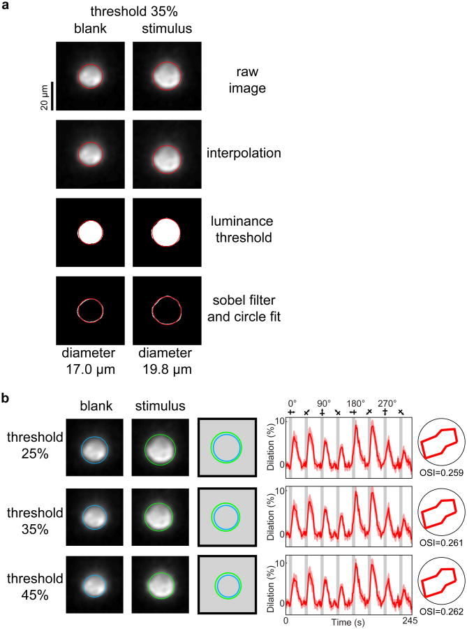
Extended Data Figure 6
Dilation measurements with circle fitting
a, The steps of the circle fitting algorithm are illustrated for a blank and a stimulus frame corresponding to the penetrating arteriole shown in the lower panel of Fig. 1b . The raw image data (first...
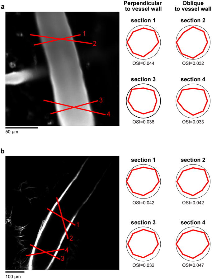
Extended Data Figure 7
Dilation measurements using the cross section algorithm do not depend on the precise location and angle of the selected cross section
a, Example cat pial artery (from Fig. 1c ) labeled with Texas-red dextran. b, Another pial artery from a different cat labelled with the artery specific dye Alexa 633. Both arteries show similar tunin...
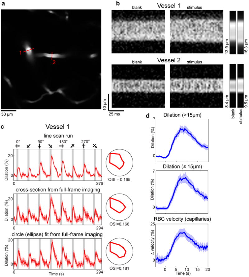
Extended Data Figure 8
Dilation measurements in small arterioles and comparison of dilation measurement techniques
a, A penetrating artery (#1, whose responses are shown in the upper panel of Fig. 1b ) and its daughter branch (#2) in cat layer 2/3 labeled with Texas-red dextran. Red lines indicate the position of ...
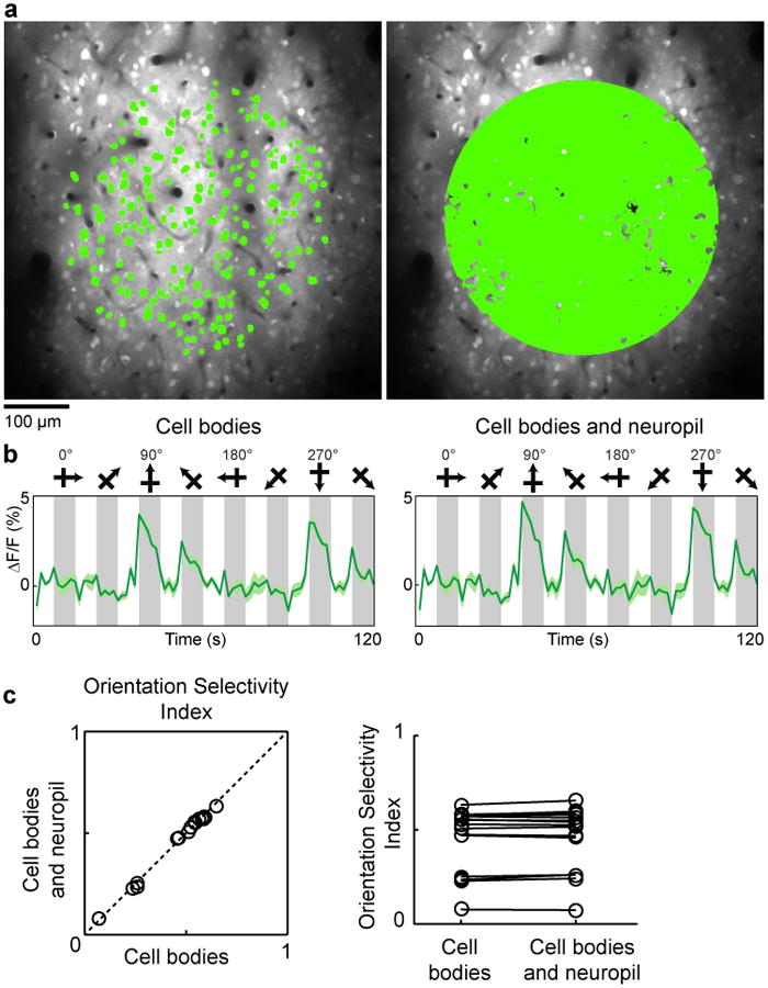
Extended Data Figure 9
Comparison of orientation selectivity in regions of calcium responses with and without neuropil
a, In vivo anatomical image of cells labeled with OGB-1 AM in cat visual cortex and selection of two different masks for quantitative analysis of orientation selectivity. Left panel: A 400-u03bcm-diam...
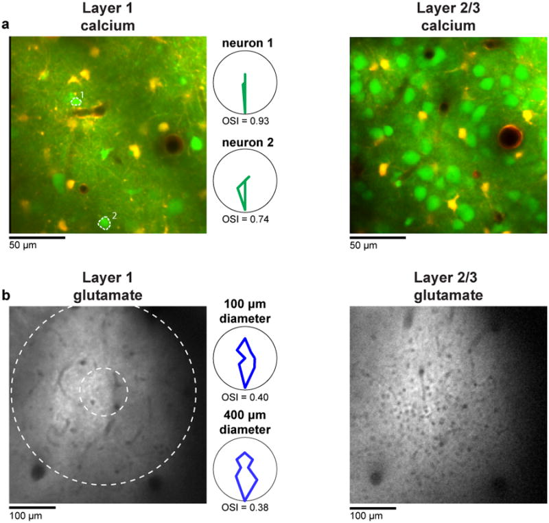
Extended Data Figure 10
Orientation selective responses in Layer 1 neurons and synapses
a, Region of cat visual cortex labeled with OGB 1-AM (to measure spiking activity) and SR101 (to distinguish astrocytes). Note the much sparser density of neuronal cell bodies in layer 1 (left) compar...
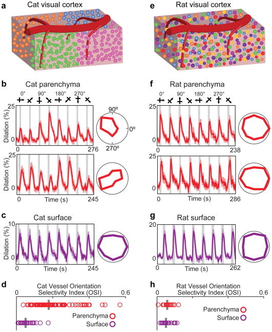
Figure 1
Selectivity of blood vessel dilation to sensory stimuli in species with and without cortical orientation maps
a, Schematic of cat visual cortex showing the columnar organization of neurons by orientation preference and a pial surface artery with multiple branches penetrating the parenchyma. Different colors o...
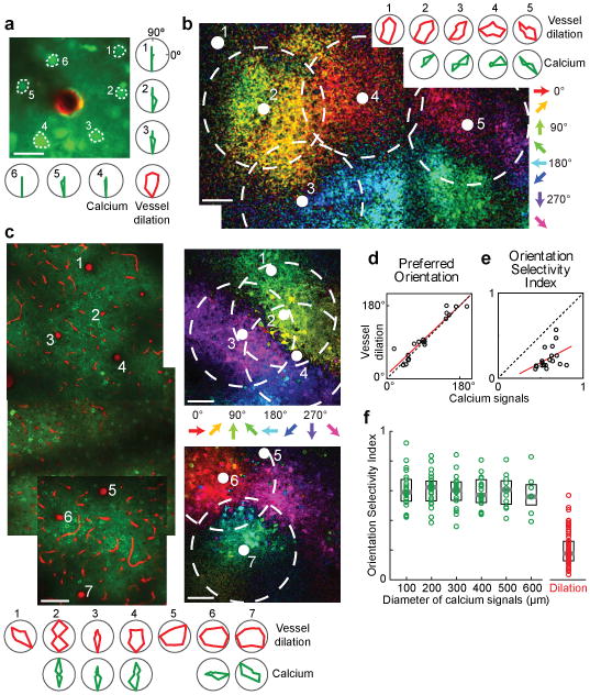
Figure 2
Stimulus selectivity of single vessels and of spiking activity in the surrounding tissue
a, In vivo anatomical image of a small region of layer 2/3 cat visual cortex labeled with OGB-1 AM (green) and an arteriole labeled with Alexa 633 (red). Polar plots show the sensory evoked calcium re...
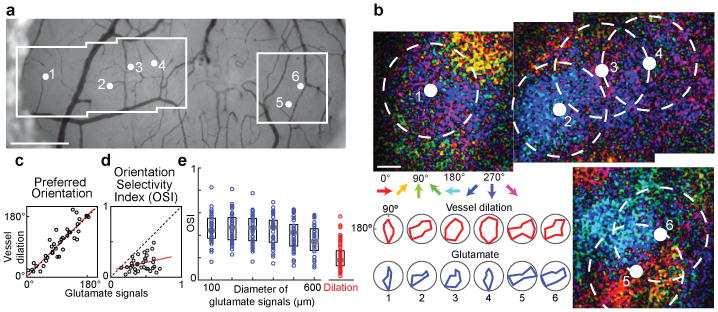
Figure 3
Stimulus selectivity of single vessels and of excitatory synaptic activity in the surrounding tissue
a, Bright field image of the surface of cat visual cortex showing the location of six penetrating arterioles and the regions targeted for two-photon imaging. b, Direction maps and polar plots of gluta...
Figure images are served from the NIH/NLM PubMed Central Open Access Subset or Europe PMC; copyright remains with the publishers and authors.
💬 Discussion
0 commentsNo comments yet. Be the first to start a discussion!
Leave a Comment