Abstract
BACKGROUND: Colour is the most important feature used in quantitative immunohistochemistry (IHC) image analysis; IHC is used to provide information relating to aetiology and to confirm malignancy. METHODS: Statistical modelling is a technique widely used for colour detection in computer vision. We have developed a statistical model of colour detection applicable to detection of stain colour in digital IHC images. Model was first trained by massive colour pixels collected semi-automatically. To speed up the training and detection processes, we removed luminance channel, Y channel of YCbCr colour space and chose 128 histogram bins which is the optimal number. A maximum likelihood classifier is used to classify pixels in digital slides into positively or negatively stained pixels automatically. The model-based tool was developed within ImageJ to quantify targets identified using IHC and histochemistry. RESULTS: The purpose of evaluation was to compare the computer model with human evaluation. Several large datasets were prepared and obtained from human oesophageal cancer, colon cancer and liver cirrhosis with different colour stains. Experimental results have demonstrated the model-based tool achieves more accurate results than colour deconvolution and CMYK model in the detection of brown colour, and is comparable to colour deconvolution in the detection of pink colour. We have also demostrated the proposed model has little inter-dataset variations. CONCLUSIONS: A robust and effective statistical model is introduced in this paper. The model-based interactive tool in ImageJ, which can create a visual representation of the statistical model and detect a specified colour automatically, is easy to use and available freely at http://rsb.info.nih.gov/ij/plugins/ihc-toolbox/index.html . Testing to the tool by different users showed only minor inter-observer variations in results.
🔬 Techniques
🧪 Sample Preparation
💻 Software Details
🏛️ Research Organizations (ROR)
Affiliated research institutions:
📋 Methods
Statistical modelling is a technique widely used for colour detection in computer vision. We have developed a statistical model of colour detection applicable to detection of stain colour in digital IHC images. Model was first trained by massive colour pixels collected semi-automatically. To speed up the training and detection processes, we removed luminance channel, Y channel of YCbCr colour space and chose 128 histogram bins which is the optimal number. A maximum likelihood classifier is used to classify pixels in digital slides into positively or negatively stained pixels automatically. The model-based tool was developed within ImageJ to quantify targets identified using IHC and histochemistry.
Methods Statistical model
The statistical model presented in [ 6 , 12 ] has been used for the detection of positive immunostain colour. For model construction, the labelled colour pixels are arranged into a colour histogram in a specific colour space. For example, in RGB colour space, the pixels are quantized into RGB colour bins. The probability of positive or negative for each bin is separately calculated as follows. 1 documentclass[12pt]{minimal} usepackage{amsmath} usepackage{wasysym} usepackage{amsfonts} usepackage{amssymb} usepackage{amsbsy} usepackage{mathrsfs} usepackage{upgreek} setlength{oddsidemargin}{-69pt} begin{document}$$begin{aligned} Prob(RGB|S)=frac{#S[RGB]}{N_{S}}quad Prob(RGB|overline{S})=frac{#overline{S}[RGB]}{N_{overline{S}}} end{aligned}$$end{document} P r o b ( R G B | S ) = # S [ R G B ] N S P r o b ( R G B | S ¯ ) = # S ¯ [ R G B ] N S ¯ In (Eq. 1 ) S is the positively stained class and documentclass[12pt]{minimal} usepackage{amsmath} usepackage{wasysym} usepackage{amsfonts} usepackage{amssymb} usepackage{amsbsy} usepackage{mathrsfs} usepackage{upgreek} setlength{oddsidemargin}{-69pt} begin{document}$$overline{S}$$end{document} S ¯ is the negatively stained class, documentclass[12pt]{minimal} usepackage{amsmath} usepackage{wasysym} usepackage{amsfonts} usepackage{amssymb} usepackage{amsbsy} usepackage{mathrsfs} usepackage{upgreek} setlength{oddsidemargin}{-69pt} begin{document}$$#S[RGB]$$end{document} # S [ R G B ] the number of positively stained pixels with a colour value of [ RGB ], documentclass[12pt]{minimal} usepackage{amsmath} usepackage{wasysym} usepackage{amsfonts} usepackage{amssymb} usepackage{amsbsy} usepackage{mathrsfs} usepackage{upgreek} setlength{oddsidemargin}{-69pt} begin{document}$$#overline{S}[RGB]$$end{document} # S ¯ [ R G B ] the number of negatively stained pixels with a colour value of [ RGB ], documentclass[12pt]{minimal} usepackage{amsmath} usepackage{wasysym} usepackage{amsfonts} usepackage{amssymb} usepackage{amsbsy} usepackage{mathrsfs} usepackage{upgreek} setlength{oddsidemargin}{-69pt} begin{document}$$N_{S}$$end{document} N S the total number of positively stained pixels and documentclass[12pt]{minimal} usepackage{amsmath} usepackage{wasysym} usepackage{amsfonts} usepackage{amssymb} usepackage{amsbsy} usepackage{mathrsfs} usepackage{upgreek} setlength{oddsidemargin}{-69pt} begin{document}$$N_{overline{S}}$$end{document} N S ¯ the total number of negatively stained pixels. Maximum likelihood The classification of this bin belongs to the target stain or the background is determined by the maximum likelihood ratio approach. 2 documentclass[12pt]{minimal} usepackage{amsmath} usepackage{wasysym} usepackage{amsfonts} usepackage{amssymb} usepackage{amsbsy} usepackage{mathrsfs} usepackage{upgreek} setlength{oddsidemargin}{-69pt} begin{document}$$begin{aligned} frac{Prob(RGB|S)}{Prob(RGB|overline{S})} ge theta quad 0 le theta le 1 end{aligned}$$end{document} P r o b ( R G B | S ) P r o b ( R G B | S ¯ ) ≥ θ 0 ≤ θ ≤ 1 The value of documentclass[12pt]{minimal} usepackage{amsmath} usepackage{wasysym} usepackage{amsfonts} usepackage{amssymb} usepackage{amsbsy} usepackage{mathrsfs} usepackage{upgreek} setlength{oddsidemargin}{-69pt} begin{document}$$theta$$end{document} θ is obtained through the experimental results presented in " Experiments and discussion " section.
Show full methods section
Statistical modelling is a technique widely used for colour detection in computer vision. We have developed a statistical model of colour detection applicable to detection of stain colour in digital IHC images. Model was first trained by massive colour pixels collected semi-automatically. To speed up the training and detection processes, we removed luminance channel, Y channel of YCbCr colour space and chose 128 histogram bins which is the optimal number. A maximum likelihood classifier is used to classify pixels in digital slides into positively or negatively stained pixels automatically. The model-based tool was developed within ImageJ to quantify targets identified using IHC and histochemistry.
Methods Statistical model
The statistical model presented in [ 6 , 12 ] has been used for the detection of positive immunostain colour. For model construction, the labelled colour pixels are arranged into a colour histogram in a specific colour space. For example, in RGB colour space, the pixels are quantized into RGB colour bins. The probability of positive or negative for each bin is separately calculated as follows. 1 documentclass[12pt]{minimal} usepackage{amsmath} usepackage{wasysym} usepackage{amsfonts} usepackage{amssymb} usepackage{amsbsy} usepackage{mathrsfs} usepackage{upgreek} setlength{oddsidemargin}{-69pt} begin{document}$$begin{aligned} Prob(RGB|S)=frac{#S[RGB]}{N_{S}}quad Prob(RGB|overline{S})=frac{#overline{S}[RGB]}{N_{overline{S}}} end{aligned}$$end{document} P r o b ( R G B | S ) = # S [ R G B ] N S P r o b ( R G B | S ¯ ) = # S ¯ [ R G B ] N S ¯ In (Eq. 1 ) S is the positively stained class and documentclass[12pt]{minimal} usepackage{amsmath} usepackage{wasysym} usepackage{amsfonts} usepackage{amssymb} usepackage{amsbsy} usepackage{mathrsfs} usepackage{upgreek} setlength{oddsidemargin}{-69pt} begin{document}$$overline{S}$$end{document} S ¯ is the negatively stained class, documentclass[12pt]{minimal} usepackage{amsmath} usepackage{wasysym} usepackage{amsfonts} usepackage{amssymb} usepackage{amsbsy} usepackage{mathrsfs} usepackage{upgreek} setlength{oddsidemargin}{-69pt} begin{document}$$#S[RGB]$$end{document} # S [ R G B ] the number of positively stained pixels with a colour value of [ RGB ], documentclass[12pt]{minimal} usepackage{amsmath} usepackage{wasysym} usepackage{amsfonts} usepackage{amssymb} usepackage{amsbsy} usepackage{mathrsfs} usepackage{upgreek} setlength{oddsidemargin}{-69pt} begin{document}$$#overline{S}[RGB]$$end{document} # S ¯ [ R G B ] the number of negatively stained pixels with a colour value of [ RGB ], documentclass[12pt]{minimal} usepackage{amsmath} usepackage{wasysym} usepackage{amsfonts} usepackage{amssymb} usepackage{amsbsy} usepackage{mathrsfs} usepackage{upgreek} setlength{oddsidemargin}{-69pt} begin{document}$$N_{S}$$end{document} N S the total number of positively stained pixels and documentclass[12pt]{minimal} usepackage{amsmath} usepackage{wasysym} usepackage{amsfonts} usepackage{amssymb} usepackage{amsbsy} usepackage{mathrsfs} usepackage{upgreek} setlength{oddsidemargin}{-69pt} begin{document}$$N_{overline{S}}$$end{document} N S ¯ the total number of negatively stained pixels. Maximum likelihood The classification of this bin belongs to the target stain or the background is determined by the maximum likelihood ratio approach. 2 documentclass[12pt]{minimal} usepackage{amsmath} usepackage{wasysym} usepackage{amsfonts} usepackage{amssymb} usepackage{amsbsy} usepackage{mathrsfs} usepackage{upgreek} setlength{oddsidemargin}{-69pt} begin{document}$$begin{aligned} frac{Prob(RGB|S)}{Prob(RGB|overline{S})} ge theta quad 0 le theta le 1 end{aligned}$$end{document} P r o b ( R G B | S ) P r o b ( R G B | S ¯ ) ≥ θ 0 ≤ θ ≤ 1 The value of documentclass[12pt]{minimal} usepackage{amsmath} usepackage{wasysym} usepackage{amsfonts} usepackage{amssymb} usepackage{amsbsy} usepackage{mathrsfs} usepackage{upgreek} setlength{oddsidemargin}{-69pt} begin{document}$$theta$$end{document} θ is obtained through the experimental results presented in " Experiments and discussion " section.
Colour models
It is recognised that Red, Green and Blue ( RGB ) colour space is not suitable for image analysis. One reason for this is that chromaticity information and brightness (luminance) information are mixed together in this colour space, and it is often desirable to process chromatic and luminance signals separately. This means that colour detection techniques often involve separating the chromaticity signal from the luminance signal. In immunostain detection, it is the chromaticity signal or the colour spectrum that is of interest rather than absolute brightness. The chromaticity signals encode the spectral information of the stain and can therefore be used to detect positive staining. From a computational perspective using a 2D chromaticity space makes it easier to model the probability density function. 3 documentclass[12pt]{minimal} usepackage{amsmath} usepackage{wasysym} usepackage{amsfonts} usepackage{amssymb} usepackage{amsbsy} usepackage{mathrsfs} usepackage{upgreek} setlength{oddsidemargin}{-69pt} begin{document}$$begin{aligned} r=frac{R}{R+G+B}quad g=frac{G}{R+G+B}quad b=frac{B}{R+G+B}end{aligned}$$end{document} r = R R + G + B g = G R + G + B b = B R + G + B 4 documentclass[12pt]{minimal} usepackage{amsmath} usepackage{wasysym} usepackage{amsfonts} usepackage{amssymb} usepackage{amsbsy} usepackage{mathrsfs} usepackage{upgreek} setlength{oddsidemargin}{-69pt} begin{document}$$begin{aligned} rg=r-gquad by=frac{r+g}{2}-b end{aligned}$$end{document} r g = r - g b y = r + g 2 - b 5 documentclass[12pt]{minimal} usepackage{amsmath} usepackage{wasysym} usepackage{amsfonts} usepackage{amssymb} usepackage{amsbsy} usepackage{mathrsfs} usepackage{upgreek} setlength{oddsidemargin}{-69pt} begin{document}$$begin{aligned} Cb=- 0.1687times R - 0.3313times G + 0.5times B end{aligned}$$end{document} C b = - 0.1687 × R - 0.3313 × G + 0.5 × B 6 documentclass[12pt]{minimal} usepackage{amsmath} usepackage{wasysym} usepackage{amsfonts} usepackage{amssymb} usepackage{amsbsy} usepackage{mathrsfs} usepackage{upgreek} setlength{oddsidemargin}{-69pt} begin{document}$$begin{aligned} Cr=0.5times R - 0.4187times G - 0.0813times B end{aligned}$$end{document} C r = 0.5 × R - 0.4187 × G - 0.0813 × B 7 documentclass[12pt]{minimal} usepackage{amsmath} usepackage{wasysym} usepackage{amsfonts} usepackage{amssymb} usepackage{amsbsy} usepackage{mathrsfs} usepackage{upgreek} setlength{oddsidemargin}{-69pt} begin{document}$$begin{aligned} Prob((rg,by)|S)=frac{#S[(rg,by)]}{N_{S}} quad Prob((rg,by)|overline{S})=frac{#overline{S}[(rg,by)]}{N_{overline{S}}} end{aligned}$$end{document} P r o b ( ( r g , b y ) | S ) = # S [ ( r g , b y ) ] N S P r o b ( ( r g , b y ) | S ¯ ) = # S ¯ [ ( r g , b y ) ] N S ¯ 8 documentclass[12pt]{minimal} usepackage{amsmath} usepackage{wasysym} usepackage{amsfonts} usepackage{amssymb} usepackage{amsbsy} usepackage{mathrsfs} usepackage{upgreek} setlength{oddsidemargin}{-69pt} begin{document}$$begin{aligned} Prob((Cb,Cr)|S)=frac{#S[(Cb,Cr)]}{N_{S}} quad Prob((Cb,Cr)|overline{S})=frac{#overline{S}[(Cb,Cr)]}{N_{overline{S}}} end{aligned}$$end{document} P r o b ( ( C b , C r ) | S ) = # S [ ( C b , C r ) ] N S P r o b ( ( C b , C r ) | S ¯ ) = # S ¯ [ ( C b , C r ) ] N S ¯ In order to demonstrate that luminance is less important than chromaticity in stain colour detection we tested four colour models, in experiment step one, only some of which used luminance information. The models tested were the RGB colour model, the opponent colour model, the YCbCr model and the CbCr model. In the opponent colour model red–green ( rg ) and blue–yellow ( by ) chromaticity signals are derived from the original RGB input (Eq. 3 ). The Cb and Cr chromaticity signals are derived from the original RGB space (Eq. 5 ). Statistical colour models in the chromaticity space can then be constructed (Eqs. 7 and 8 ).
Step two: comparison of the statistical colour detection method with other methods Dataset The dataset used in the comparative study was the same as that used in the robustness evaluation reported in previous experiment. Experiment In this study we compared the statistical method with two previously developed colour detection methods in widespread use [ 9 , 10 ]. All the methods were trained and tested based on the same datasets, which were prepared from different types of images of IHC staining. We compared the terms of detection accuracy, separation of stain colours, and variations between user trained models and vectors. Accuracy of colour detection in DAB-stained samples Table 2 10 CD vectors obtained from 5 WS training images and 5 TMA training images for brown colour detection Images Whole slide TMA R G B R G B 1 0.44950655 0.60628647 0.65601873 0.5197582 0.60258 0.6055978 2 0.44893575 0.6022728 0.6600941 0.52838445 0.5891207 0.6113483 3 0.40408775 0.6007869 0.6897595 0.55297637 0.5856209 0.5926764 4 0.39064342 0.5893953 0.70711446 0.4932045 0.59396774 0.6355719 5 0.37070048 0.5971876 0.7113003 0.5172909 0.59305906 0.6170017 The average results from four users using the new method were compared with results obtained from colour deconvolution (CD) and CMYK models. The study was conducted in ImageJ. Colour deconvolution was programmed by Landini as a plugin for ImageJ [ 14 ] based on the National Institutes of Health Image macro. Instead of using single DAB-stained sample, we trained the CD vectors by the same 10 training samples, 5 WS images and 5 TMA images in mixed set, as used in previous experiment. Vectors for brown colour of DAB stain were obtained through ImageJ Plugin. Each vector was obatined from one training image. They were tested by the corresponding test images. The results were shown in Table 2 . The results with the 10 vectors obtained in this way were much worse than those obtained with the built-in H-DAB vector ( documentclass[12pt]{minimal} usepackage{amsmath} usepackage{wasysym} usepackage{amsfonts} usepackage{amssymb} usepackage{amsbsy} usepackage{mathrsfs} usepackage{upgreek} setlength{oddsidemargin}{-69pt} begin{document}$$R = 0.26814753, G = 0.57031375, B = 0.77642715$$end{document} R = 0.26814753 , G = 0.57031375 , B = 0.77642715 ) (see Fig. 5 ); we therefore used the built-in vector to discriminate the brown colour from the background in the evaluation. The CMYK model was also developed in ImageJ based on the functions mentioned in [ 15 ]. Fig. 6 ROC curves of CD, CMYK, mean value of ST with three sets of training samples. Colour Deconvolution CD , CMYK colour space CMYK , mean value of ST models trained from corresponding images CorrAvg , mean value of ST models trained from mixed training images MixAvg , mean value of ST models trained from WS (TMA) training images WS(TMA)Avg . The plot at the top shows the ROC curves for CD ( red dashed line ), CMYK ( brown dotted line ), the mean value of ST models with corresponding training images ( smooth green line ), the mean value of ST models with mixed training images ( smooth purper line ), and the mean value of ST models with TMA training images ( smooth blue line ) on 50 WS test images; the plot at the bottom shows the ROC curves for CD, CMYK and the mean value of ST models with three sets of traning images (WS, Mixed and TMA training images) on 50 TMA test images. The horizontal axis is false-positive ratio and vertical axis is true-positive ratio As shown in Fig. 6 , both in WS and TMA datasets, almost methods produced highly accurate results. Statistical models with corresponding training images and CD with built-in vector were achieving close to 100 percent true-positive rate. The mean values of the statistical models, achieved the best results over the 50 WS test images, with a false-positive rate of 8.3 %; the false-positive rate 12.0 % for the CD method. The CMYK model had the lowest rate, true-positive rate, 92.9 %. The statistical models also achieved the best result for the set of 50 TMA test images, a 14.9 % false-positive rate compared with 16.6 % for the CD method. Again the CMYK model had the lowest true-positive rate, 91.4 %. Table 3 The AUC values of the ROC curves of 12 models, when false positive ratio equals 10 % Whole slide TMA Model (WS) (%) Model (TMA) (%) Model (mix) (%) Model (WS) (%) Model (TMA) (%) Model (mix) (%) User1 97.2 97.0 97.1 95.8 95.9 95.9 User2 97.2 97.1 97.1 95.8 95.9 95.9 User3 97.0 96.9 94.6 95.8 96.6 96.6 User4 96.9 96.9 96.9 96.6 96.6 96.6 AVG 97.1 97.0 96.5 96.0 96.2 96.2 CD 93.9 94.5 CMYK 86.1 69.3 WS whole slide test images; TMA TMA test images; ST ( WS ) statistical model constructed on 10 WS training images; ST ( TMA ) statistical model constructed on 10 TMA training images; Mix statistical model constructed on 10 mixed training images (5 WS images and 5 TMA images); AVG average values of four user-detected results; CD colour deconvolution To clarify these results, we calculated AUROC (area under ROC curve). Table 3 shows that the statistical colour models produced the best results. CD produced much better results than CMYK on both WS and TMA test images. Table 2 also shows that the user-generated models had varied slightly in terms of detection accuracy. For example, for brown colour detection, the lowest AUC was 94.6 % and the maximum was 97.2 %. These results indicate that models generated by different users using this tool are all highly accurate and therefore that the method is robust and fairly user-independent. However, CD method with trained vectors has obvious variations in detection results, especially in detection of DAB stained TMA images, see Fig. 5 . The results also show the mixed models and models constructed not from corresponding training images can generate similar results to the models only trained by corresponding training images. It demostrates the model constructed by the whole range of colour shades can be adopted in different datasets obtained from different diseases for the same stain colour detection. Dark stain colour detection Fig. 7 The statistical model detected stain colour on IHC stained samples. a , b columns are the DAB-stained samples from WS images; c , d columns are the DAB-stained samples from TMA images; e column is a PSR-stained liver cirrhosis sample; f column is a DAB-stained liver cirrhosis sample showing elastin fibrosis. The images in top row are original IHC stained images; the images in middle row are model-detected brown or pink colour ; the bottom row is model-detected counter stain colour, blue or yellow Normal brown colour was detected easily and separated from the background by all three methods. Detection of brown coloration in a dark-stained slide is more challenging however; the CMYK method undercounted dark brown-coloured pixels (Fig. 1 d, e) whereas CD falsely detected dark brown as the colour blue (Fig. 1 b, c). This evaluation of CMYK demonstrated that a colour space-based method performed less accurately in stain colour detection [ 16 ]. Classification of multi-stain colours in colour space may be affected by overlap. The CD method also suffers from this problem and the non-linear light absorption of DAB stain. The statistically-based interactive tool detected dark brown and blue correctly (see Fig. 7 ).
📊 Figures
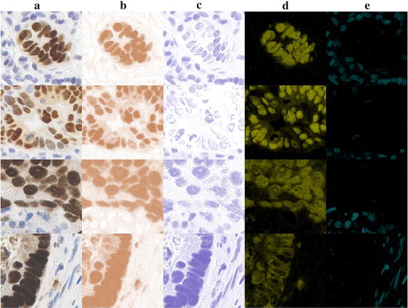
Fig. 1
The previous methods detected stain colour on DAB stained samples. a Column is the original DAB stained samples, the upper two samples from WS images and lower two samples from TMA images; b , c colum...
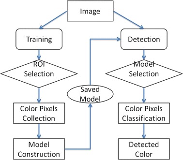
Fig. 2
Workflow of stain colour detection in the interactive tool
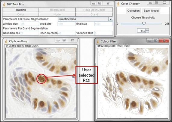
Fig. 3
Stain colour detection in toolbox. This is an illustration of the training phase of colour detection. The left image is the original image. The right image is the output image. The colour pixels in th...
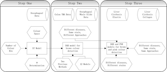
Fig. 4
Flowchart of three steps of statistical model test
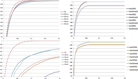
Fig. 5
ROC curves for different user constructed statistical models. The plot at the top left is ROC curves for user obtained 5 vectors (based on 5 WS images) on 50 WS test images; The plot at the bottom lef...
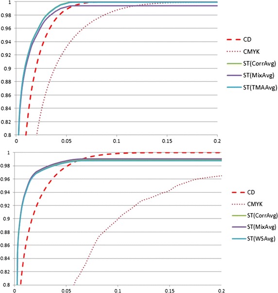
Fig. 6
ROC curves of CD, CMYK, mean value of ST with three sets of training samples. Colour Deconvolution CD , CMYK colour space CMYK , mean value of ST models trained from corresponding images CorrAvg , mea...
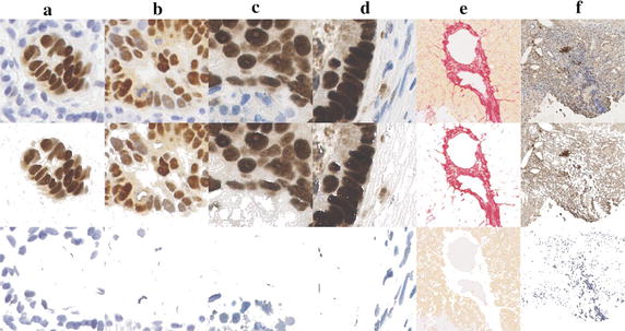
Fig. 7
The statistical model detected stain colour on IHC stained samples. a , b columns are the DAB-stained samples from WS images; c , d columns are the DAB-stained samples from TMA images; e column is a P...
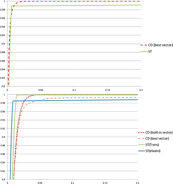
Fig. 8
ROC curves for CD and ST model for the PSR and elastin datasets. Plot at the top is the ROC for pink colour detection on PSR stained images, the ROC curve for CD with best-vector (CD(best-vector)) is ...
Figure images are served from the NIH/NLM PubMed Central Open Access Subset or Europe PMC; copyright remains with the publishers and authors.
💬 Discussion
0 commentsNo comments yet. Be the first to start a discussion!
Leave a Comment