Abstract
Single-particle cryo-electron microscopy (cryo-EM) has become a powerful technique in the field of structural biology. However, the inability to reliably produce pure, homogeneous membrane protein samples hampers the progress of their structural determination. Here, we develop a bottom-up iterative method, Build and Retrieve (BaR), that enables the identification and determination of cryo-EM structures of a variety of inner and outer membrane proteins, including membrane protein complexes of different sizes and dimensions, from a heterogeneous, impure protein sample. We also use the BaR methodology to elucidate structural information from Escherichia coli K12 crude membrane and raw lysate. The findings demonstrate that it is possible to solve high-resolution structures of a number of relatively small (<100 kDa) and less abundant (<10%) unidentified membrane proteins within a single, heterogeneous sample. Importantly, these results highlight the potential of cryo-EM for systems structural proteomics.
🔬 Techniques
🧬 Organisms
🔬 Cell Lines
🏭 Microscope Brands
🧪 Reagent Suppliers
📷 Detectors
💻 Software Details
💾 Data Repositories
🏛️ Research Organizations (ROR)
Affiliated research institutions:
📋 Methods
“Build and Retrieve” (BaR) methodology BaR is a bottom-up systems structural proteomic approach to identify and obtain near atomic structural models of multiple proteins from raw samples, including crude membranes and cell lysates ( Figure 1 ). Here, we demonstrate that it is possible to simultaneously and rapidly determine several protein structures from a single, heterogeneous sample. Step 1: Sample preparation. For raw cell membranes, we solubilize the membranes using detergent and reconstitute the solubilized membrane proteins into lipidic nanodiscs from endogenous sources. We then separate and enrich the protein-nanodisc complexes from empty nanodiscs using size exclusion chromatography. For raw cell lysates, we use size exclusion chromatography to enrich protein samples from endogenous sources. Step 2: Cryo-EM imaging and processing. We perform data collection and initial imaging processing under standard cryo-EM protocols that are described in the Online Methods. We apply a combination of blob picker followed by 2D classification using a subset of micrographs to generate initial particle templates. We then employ template picker to pick the entire dataset, giving rise to the full particle set. Step 3: Initial 2D classification. We perform in silico purification of the full particle set using several rounds of 2D classification. Owing to the heterogeneous nature of the sample, it is not possible to clearly separate particle classes based on results from 2D classification. Therefore, all classes with distinct structural features are selected for continued processing. Step 4: Preliminary 3D classification. Next, we sort the full particle set using 2D and 3D ab initio classifications to divide the complete particle set into subsets with similar structural features. Different starting 3D classes for ab initio classification are trialed based on the number of resulting converged classes. After this initial 3D classification, different subsets are treated as separate entities for Step 5. Step 5: “Build” initial maps. The subsets of selected classes from step 4 are rigorously cleaned and re-sorted through several rounds of 2D classification. Only classes showing clear high-resolution features are selected. A combination of ab initio and heterogeneous 3D classification are used to clean the resulting particles. Initial maps are solved using non-uniform refinement with C1 symmetry. Step 6: “Retrieve” full particle sets. Owing to the rigorous cleaning procedures performed in Step 5, all reconstructions suffer from incomplete views. To increase particle counts and obtain more views for each biomacromolecule, the “built” maps from Step 5 are used as templates for 3D heterogeneous classification of the 2D cleaned particles from Step 3, where each subset is treated separately for final structural refinement. This procedure is vital in “retrieving” enough information and particles for near atomic resolution reconstruction. Step 7: Final refinement. Newly retrieved subsets are then cleaned using multiple rounds of 2D and 3D classifications. Non-uniform refinement is used to build the final maps. Symmetry can be applied at this step to enhance the resolution. These near atomic resolution cryo-EM maps can now be used to determine the identities of biomacromolecules using phenix.sequence_from_map implemented in the PHENIX suite 5 . The protein models are then built using Coot 6 and refined using PHENIX 5 . Step 8: Mass spectrometry. Mass spectrometry, such as native mass spectrometry (nMS) and proteomics, are used to confirm the presence of these proteins.
Show full methods section
“Build and Retrieve” (BaR) methodology BaR is a bottom-up systems structural proteomic approach to identify and obtain near atomic structural models of multiple proteins from raw samples, including crude membranes and cell lysates ( Figure 1 ). Here, we demonstrate that it is possible to simultaneously and rapidly determine several protein structures from a single, heterogeneous sample. Step 1: Sample preparation. For raw cell membranes, we solubilize the membranes using detergent and reconstitute the solubilized membrane proteins into lipidic nanodiscs from endogenous sources. We then separate and enrich the protein-nanodisc complexes from empty nanodiscs using size exclusion chromatography. For raw cell lysates, we use size exclusion chromatography to enrich protein samples from endogenous sources. Step 2: Cryo-EM imaging and processing. We perform data collection and initial imaging processing under standard cryo-EM protocols that are described in the Online Methods. We apply a combination of blob picker followed by 2D classification using a subset of micrographs to generate initial particle templates. We then employ template picker to pick the entire dataset, giving rise to the full particle set. Step 3: Initial 2D classification. We perform in silico purification of the full particle set using several rounds of 2D classification. Owing to the heterogeneous nature of the sample, it is not possible to clearly separate particle classes based on results from 2D classification. Therefore, all classes with distinct structural features are selected for continued processing. Step 4: Preliminary 3D classification. Next, we sort the full particle set using 2D and 3D ab initio classifications to divide the complete particle set into subsets with similar structural features. Different starting 3D classes for ab initio classification are trialed based on the number of resulting converged classes. After this initial 3D classification, different subsets are treated as separate entities for Step 5. Step 5: “Build” initial maps. The subsets of selected classes from step 4 are rigorously cleaned and re-sorted through several rounds of 2D classification. Only classes showing clear high-resolution features are selected. A combination of ab initio and heterogeneous 3D classification are used to clean the resulting particles. Initial maps are solved using non-uniform refinement with C1 symmetry. Step 6: “Retrieve” full particle sets. Owing to the rigorous cleaning procedures performed in Step 5, all reconstructions suffer from incomplete views. To increase particle counts and obtain more views for each biomacromolecule, the “built” maps from Step 5 are used as templates for 3D heterogeneous classification of the 2D cleaned particles from Step 3, where each subset is treated separately for final structural refinement. This procedure is vital in “retrieving” enough information and particles for near atomic resolution reconstruction. Step 7: Final refinement. Newly retrieved subsets are then cleaned using multiple rounds of 2D and 3D classifications. Non-uniform refinement is used to build the final maps. Symmetry can be applied at this step to enhance the resolution. These near atomic resolution cryo-EM maps can now be used to determine the identities of biomacromolecules using phenix.sequence_from_map implemented in the PHENIX suite 5 . The protein models are then built using Coot 6 and refined using PHENIX 5 . Step 8: Mass spectrometry. Mass spectrometry, such as native mass spectrometry (nMS) and proteomics, are used to confirm the presence of these proteins.
Online Methods
Cloning, expression and purification of B. pseudomallei HpnN Briefly, the full-length BpHpnN membrane protein containing a 6xHis tag at the C-terminus was overproduced in E. coli BL21(DE3) ΔacrB cells, which harbors a deletion in the chromosomal acrB gene, generating pET15bΩ hpnN . Cells were grown in 6 l of LB medium with 100 μg/ml ampicillin at 37°C. When the OD 600 nm reached 0.5, the culture was treated with 0.2 mM isopropyl-β-D-thiogalactopyranoside (IPTG) to induce hpnN expression, and cells were harvested within 4 h. The collected bacteria were resuspended in low salt buffer containing 100 mM sodium phosphate (pH 7.2), 10 % glycerol, 1 mM ethylenediaminetetraacetic acid (EDTA) and 1 mM phenylmethylsulfonyl fluoride (PMSF), and then disrupted with a French pressure cell. The membrane fraction was collected and washed twice with high salt buffer containing 20 mM sodium phosphate (pH 7.2), 2 M KCl, 10 % glycerol, 1 mM EDTA and 1 mM PMSF, and once with final buffer containing 20 mM HEPES-NaOH buffer (pH 7.5) and 1 mM PMSF as described previously 32 . The membrane protein was then solubilized in 2% (w/v) n-dodecyl-β-D-maltoside (DDM). Insoluble material was removed by ultracentrifugation at 100,000 x g. The extracted protein was then purified using a Ni 2+ -affinity column. The purified protein was concentrated to 10 mg/ml in a buffer containing 20 mM Tris-HCl (pH 7.5), 100 mM NaCl and 0.05% DDM.
Nanodisc preparation
To assemble BpHpnN into nanodiscs, a mixture containing 10 μM BpHpnN, 30 μM MSP (1E3D1) and 900 μM E. coli total extract lipid was incubated for 15 minutes at room temperature. After, 0.8 mg/ml pre-washed Bio-beads (Bio-Rad) was added. The resultant mixture was incubated for 1 hour on ice followed by overnight incubation at 4°C. The protein-nanodisc solution was filtered through 0.22 μm nitrocellulose-filter tubes to remove the Bio-beads. A Superose 6 column (GE Healthcare) equilibrated with 20 mM Tris-HCl, pH 7.5, and 100 mM NaCl was then used to separate free nanodiscs from the BpHpnN-nanodisc complex. Fractions corresponding to the size of the monomeric BpHpnN-nanodisc complex were collected for cryo-EM study. E. coli K12 crude cell membrane E. coli K12 cells (strain BW25113) (Yale CGSC) were grown in 1 l of LB medium at 37°C and harvested when the OD 600 nm reached 1.2. The collected cells were resuspended in buffer containing 100 mM sodium phosphate (pH 7.2) and 10 % glycerol, and disrupted with a French pressure cell. The membrane fraction was collected, resuspended in buffer containing 20 mM Tris-HCl (pH 7.5) and 100 mM NaCl, and solubilized in 1% (w/v) DDM. Insoluble material was removed by ultracentrifugation at 100,000 x g. The extracted cell membrane contained a variety of unknown membrane proteins. The procedures for assembling these membrane proteins into nanodiscs were the same as those for the BpHpnN sample as described above. The processes of separating the protein-nanodisc complexes from empty nanodiscs and enriching these protein complexes were done using a Superose 6 column (GE Healthcare) equilibrated with 20 mM Tris-HCl, pH 7.5, and 100 mM NaCl. E. coli K12 raw cell lysate E. coli K12 cells (strain BW25113) (Yale CGSC) were grown in 1 l of LB medium at 37°C and harvested when the OD 600 nm reached 1.2. The collected cells were resuspended in buffer containing 20 mM Tris-HCl (pH 7.5) and 100 mM NaCl, and disrupted with a French pressure cell. Insoluble material from the cell lysate was removed by ultracentrifugation at 100,000 x g. The extracted cell lysate, containing a variety of unknown periplasmic and cytoplasmic proteins, was enriched using a Superose 6 column (GE Healthcare) equilibrated with 20 mM Tris-HCl, pH 7.5, and 100 mM NaCl. Electron microscopy sample preparation and data collection The BpHpnN, E. coli K12 membrane and E. coli K12 cell lysate samples were concentrated to 0.7 mg/ml, 1 mg/ml and 1 mg/ml, respectively. These samples were applied to glow-discharged holey carbon grids (Quantifoil Cu R1.2/1.3, 300 mesh), blotted for 5 s, 7 s and 7 s, respectively, and then plunge-frozen in liquid ethane using a Vitrobot (Thermo Fisher). The grids were transferred into cartridges. A Titan Krios cryo-electron transmission microscope (Thermo Fisher) was used to collect cryo-EM images. The images were recorded at 1-2.5 μm defocus on a K3 direct electron detector (Gatan) with super-resolution mode at a physical pixel size of 1.08 Å/phys. pixel (super resolution 0.54 Å/pixel). For the BpHpnN sample, each micrograph was exposed for 3.2 s with 18.2 e − /sec/phys. pixel dose rate (total specimen dose, 50 e − /A 2 ). 40 frames were captured per specimen area using Latitude (Gatan, Pleasanton, CA). A total of 13,093 images were recorded and processed. For the E. coli K12 cell membrane and cell lysate samples, 7,643 and 5,067 movies were collected over 42 frames (4.2 s exposure time; 11.97 e − /sec/phys. pixel dose rate; 40 e − /A 2 total dose) in SerialEM 33 , respectively. Data processing The BpHpnN, E. coli K12 crude cell membrane and E. coli K12 raw cell lysate were processed separately using an identical protocol. Super-resolution image stacks were aligned and binned by 2 using MotionCor2 34 to give a final pixel size of 1.08 Å/pixel. CTFs were estimated using patch CTF in cryoSPARC 35 . After manual inspection to discard poor images and estimate particle size, the blob picker in cryoSPARC 35 was used to select particles from subsets of micrographs. These particles were classified with one round of 2D classification and clear templates were selected for template picking in cryoSPARC 35 . Template picker was used to select initial particle sets. Several iterative rounds of 2D classifications were used to clean these particle sets with different circular masks to account for different particle sizes. Featureless classes were removed from each step, resulting in cleaned heterogeneous particle stacks for further processing. From these cleaned heterogeneous particle sets, particles were classified and final maps were solved using an iterative method termed “Build and Retrieve” (BaR) processing (which is summarized in Extended Data Figure 1 , Supplementary Figure 1 and Supplementary Figure 4 ). Briefly, ab initio methods were used to “build” initial 3D maps from the complete dataset and particles were then “retrieved” based on the maps. To build the initial maps, particles were separated using 2D classification paired with 3D ab initio and heterogeneous classifications. The combination of these techniques was used to divide the dataset into subsets with similar structural features. Each subset was then treated as an individual particle set, where several rounds of 2D classification followed by 3D ab initio reconstruction were used to improve the quality of each subset. Non-uniform refinement was applied to “build” the preliminary maps. To increase particle counts, these initial maps were used to “retrieve” particles from the cleaned heterogeneous particle stack. 3D heterogeneous refinement using the ab initio maps, determined from the “build” phase of BaR, was applied to the cleaned heterogeneous particle sets. The new particle subsets were then cleaned using multiple rounds of 2D and 3D ab initio classifications. Non-uniform refinement using cryoSPARC 35 with symmetry imposed was used to refine all symmetrical protein structures, while non-uniform refinement followed by local refinement with non-uniform sampling was used to refine those protein structures without a distinct symmetry. The maps were further processed using cryo-EM density modification 36 in PHENIX 5 , which enhanced the quality of the maps. The quality of the maps corresponding to all of these different proteins was excellent, enabling us to trace most of the Cα atoms in these protein molecules. The main-chain (Cα) of these proteins were manually traced using the program Coot 6 . The phenix.sequence_from_map program in PHENIX 5 was then used to generate the best-fitting sequences. The identities of these proteins were revealed based on the protein sequences, and their presence was further confirmed by nMS and proteomics.
Model building and refinement
Model buildings of cytochrome bo 3 , BpHpnN, OmpF, SQR, OmpC, KatG and GadB were based on the cryo-EM maps generated from the BaR methodology. The subsequent model rebuilding processes were performed using Coot 6 . Structure refinements were done using the phenix.real_space_refine program 37 from the PHENIX suite 5 . The final atomic models were evaluated using MolProbity 38 . The statistics associated with data collection, 3D reconstruction and model refinement are included in Supplementary Tables 1 , 2 and 4 . Native mass spectrometry Before MS analysis, the protein sample was buffer exchanged into 200 mM ammonium acetate pH 8.0 and 0.05% LDAO using a Biospin-6 (BioRad) column and introduced directly into the mass spectrometer using gold-coated capillary needles (prepared in-house). Data were collected on a Q-Exactive UHMR mass spectrometer (Thermo Fisher Scientific). The instrument parameters were as follows: capillary voltage 1.1 kV, S-lens RF 100%, quadrupole selection from 1,000 to 20,000 m/z range, collisional activation in the HCD cell 200 V, trapping gas pressure 7.5, temperature 200 °C, resolution of the instrument 12,500. The noise level was set at 3 rather than the default value of 4.64. No in-source dissociation was applied. Data were analyzed using Xcalibur 4.2 (Thermo Scientific) and UniDec 39 software packages. Protein identification by proteomics For protein identification, tryptic peptides were obtained by either digesting the protein sample directly with trypsin overnight at 37°C, or the proteins were first separated on an SDS-PAGE gel and subsequently treated with trypsin overnight at 37°C 40 . Peptides were resuspended with 0.1% formic acid and separated by nano-flow reversed-phase liquid chromatography coupled to a Q Exactive Hybrid orbitrap mass spectrometer (Thermo Fisher Scientific). The peptides were trapped onto a C18 PepMap 100 pre-column (inner diameter 300 μm × 5 mm, 100 Å; Thermo Fisher Scientific) using solvent A (0.1% formic acid in water) and separated on an analytical column (75 μm i.d. packed in-house with ReproSil-Pur 120 C18-AQ, 1.9 μm, 120 Å, Dr Maisch GmbH) using a linear gradient from 7 to 30% of solvent B (0.1% formic acid in acetonitrile) for 30 min, at a flow rate of 200 nl/min. The raw data were acquired on the mass spectrometer in a data-dependent mode. Typical mass spectrometric conditions were: spray voltage of 2.1 kV, capillary temperature of 320°C. MS spectra were acquired in the orbitrap (m/z 350–2000) with a resolution of 70,000 and an automatic gain control (AGC) target at 3 × 10e6 with a maximum injection time of 50 ms. After the MS scans, the top 10 most intense ions were selected for HCD fragmentation at an AGC target of 50,000 with maximum injection time of 120 ms. Raw data files were processed for protein identification using MaxQuant (version 1.5.0.35) and searched against the UniProt database (taxonomy filter E. coli ), precursor mass tolerance was set to 20 ppm and MS/MS tolerance to 0.05 Da. Peptides were defined to be tryptic with a maximum of two missed cleavage sites. Protein and peptide spectral match false discovery rate was set at 0.01.
Supplementary Material 1
📊 Figures
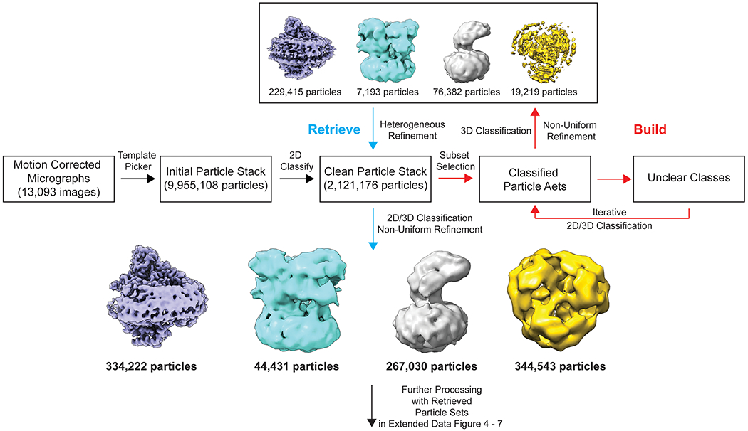
Extended Data Figure 1.
Flowchart of the u201cBuild and Retrieveu201d (BaR) iterative method for the BpHpnN sample.
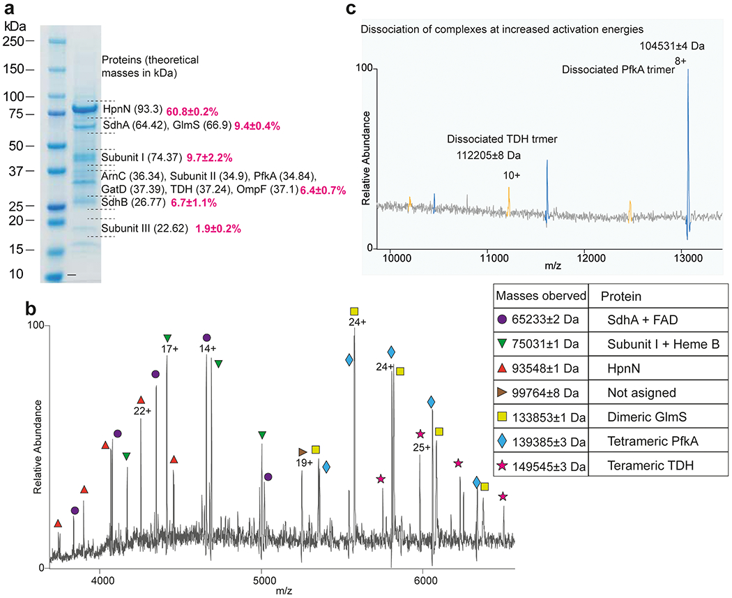
Extended Data Figure 2.
Native mass spectrometry (nMS) and proteomics analysis suggest that the sample of B. pseudomallei HpnN (BpHpnN) was co-purified with several other proteins. (a) SDS-PAGE of the purified sample where t...
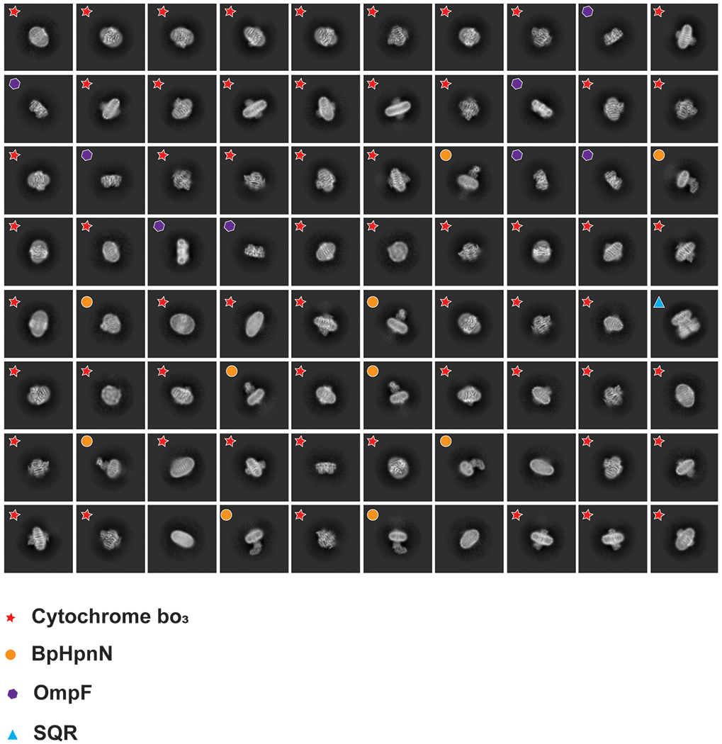
Extended Data Figure 3.
2D classes of the cryo-EM images. The 2D classification indicates that there are at least five different proteins coexisting in the nanodisc sample.
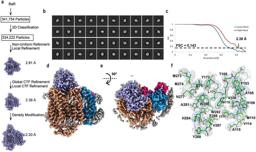
Extended Data Figure 4.
Cryo-EM analysis of the E. coli cytochrome bo 3 complex. (a) BaR processing flowchart. (b) Representative 2D classes. (c) Fourier Shell Correlation (FSC) curves. (d) Sharpened cryo-EM map of the cytoc...
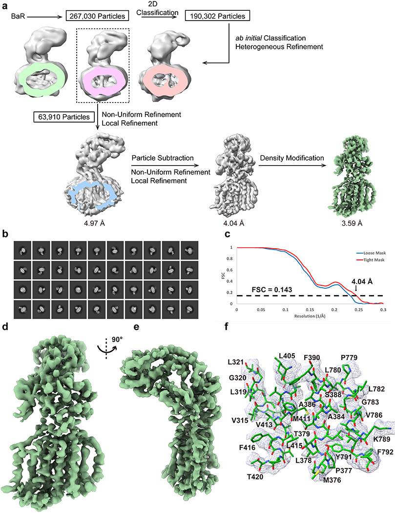
Extended Data Figure 5.
Cryo-EM analysis of the B. pseudomallei HpnN transporter. (a) BaR processing flowchart. (b) Representative 2D classes. (c) Fourier Shell Correlation (FSC) curves. (d and e) Sharpened cryo-EM maps of t...
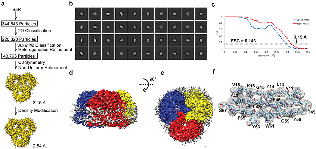
Extended Data Figure 6.
Cryo-EM analysis of the E. coli OmpF porin channel. (a) BaR processing flowchart. (b) Representative 2D classes. (c) Fourier Shell Correlation (FSC) curves. (d) Sharpened cryo-EM map of the OmpF porin...
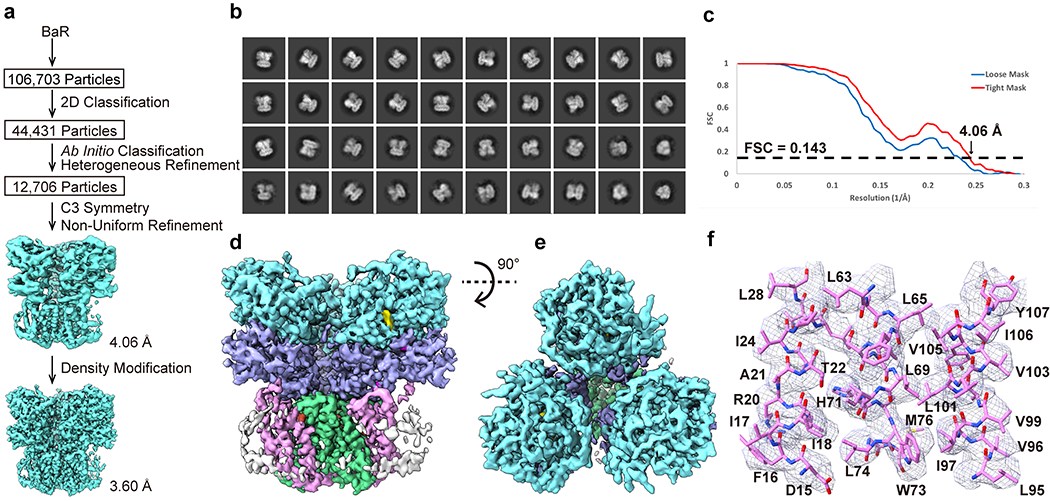
Extended Data Figure 7.
Cryo-EM analysis of the E. coli SQR complex. (a) BaR processing flowchart. (b) Representative 2D classes. (c) Fourier Shell Correlation (FSC) curves. (d) Sharpened cryo-EM map of the SQR complex viewe...
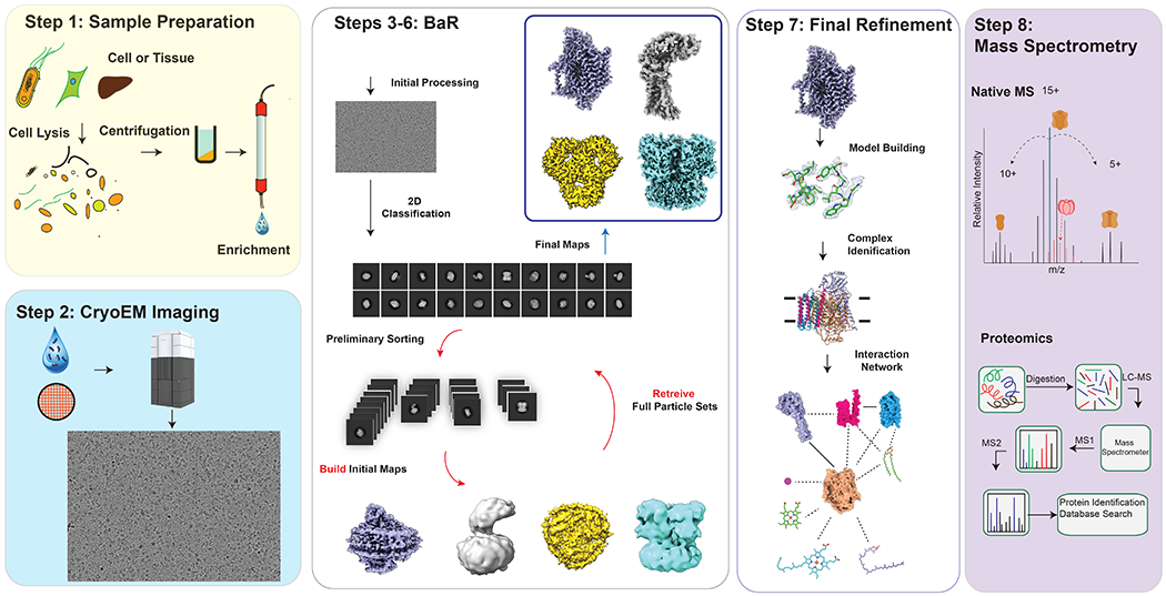
Fig. 1.
Build and Retrieve (BaR) methodology.
Protein samples are enriched by size extrusion chromatography. Cryo-EM imaging and data processing yield near atomic resolution cryo-EM maps. The data processing procedures of BaR involve extensive 2D...
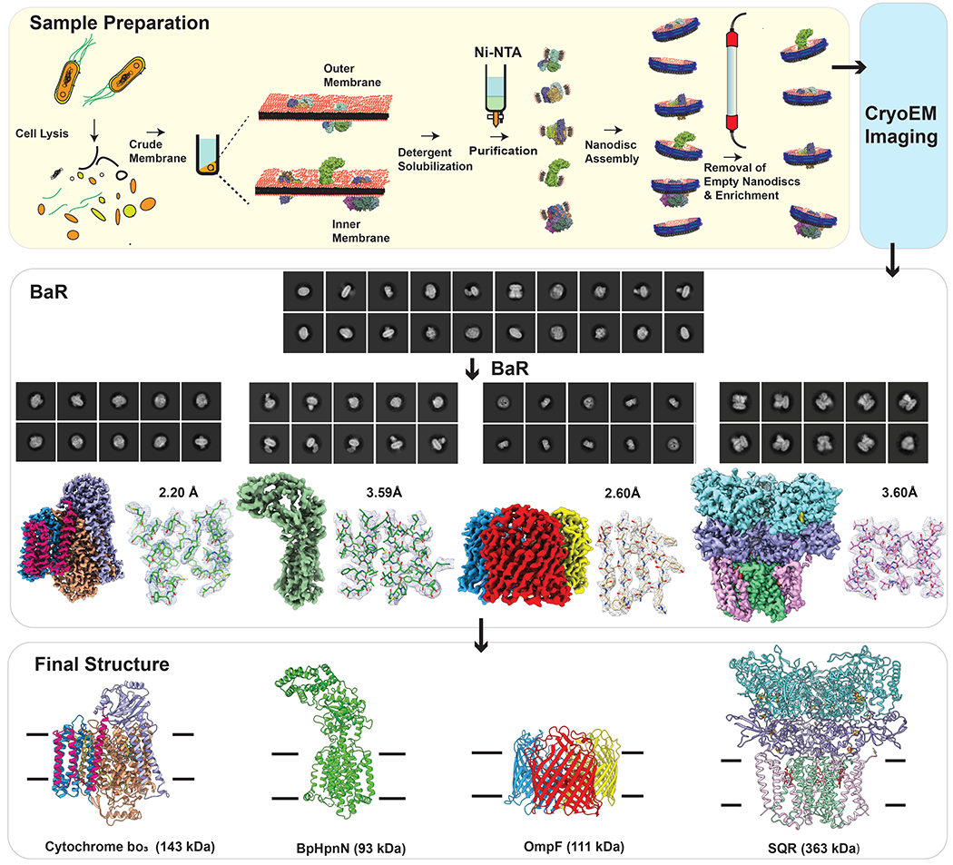
Fig. 2.
Cryo-EM structures of proteins from the heterogeneous BpHpnN membrane protein sample.
The BaR methodology was used to constructed near atomic resolution cryo-EM density maps, which allowed for the identification of the cytochrome bo 3 oxidase complex, the BpHpnN hopanoid transporter, t...
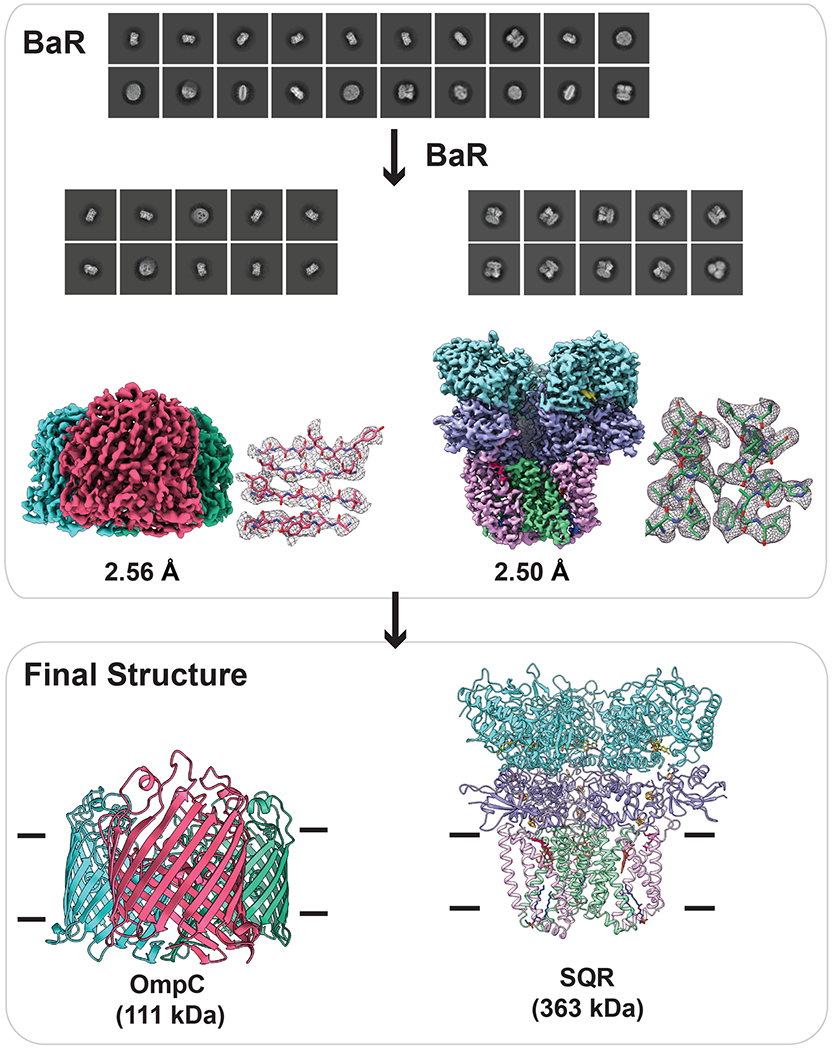
Fig. 3.
Cryo-EM structures of proteins enriched directly from E. coli crude cell membrane.
The two cryo-EM density maps were constructed to 2.56-u00c5 and 2.50-u00c5 resolutions, which allowed for the identification of the OmpC porin channel and the SQR complex, respectively.
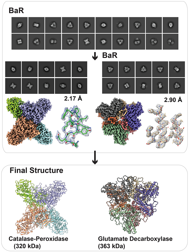
Fig. 4.
Cryo-EM structures of proteins enriched directly from E. coli raw cell lysate.
The two cryo-EM density maps were constructed to 2.17-u00c5 and 2.90-u00c5 resolutions, which allowed for the identification of the enzymes KatG catalase-peroxidase and GadB glutamate decarboxylase, r...
Figure images are served from the NIH/NLM PubMed Central Open Access Subset or Europe PMC; copyright remains with the publishers and authors.
💬 Discussion
0 commentsNo comments yet. Be the first to start a discussion!
Leave a Comment