Abstract
A fluorescent emitter simultaneously transmits its identity, location, and cellular context through its emission pattern. We developed smNet, a deep neural network for multiplexed single-molecule analysis to retrieve such information with high accuracy. We demonstrate that smNet can extract three-dimensional molecule location, orientation, and wavefront distortion with precision approaching the theoretical limit, and therefore will allow multiplexed measurements through the emission pattern of a single molecule.
🔬 Techniques
✨ Fluorophores
🧪 Sample Preparation
🔬 Cell Lines
🏭 Microscope Brands
🧪 Reagent Suppliers
📷 Detectors
🔎 Objectives
🎨 Filters
💻 Software Details
💻 Code & Software
💾 Data Repositories
🏛️ Research Organizations (ROR)
Affiliated research institutions:
📋 Methods
Optical Setup
All experimental data (except for complex PSFs and wavefront estimation data) were recorded on a custom-built single molecule switching nanoscopy (SMSN) setup built around an Olympus IX-73 microscope stand (IX-73, Olympus America Inc., Waltham, MA) with a 100×/1.35 NA silicone oil-immersion objective lens (FV-U2B714, Olympus America Inc.), a 405 nm laser (DL-405-100, CrystaLaser, Reno, NV) and a 642 nm laser (2RU-VFL-P-2000-642-B1R, MPB Communications Inc.) for activation and excitation, respectively. The filter turret contains a dichroic mirror (Di03-R405/488/561/635-t1, Semrock Inc.). A deformable mirror (MultiDM-3.5, Boston Micromachines, Cambridge, MA) placed at the conjugated pupil plane is used for correcting systematic aberrations and introducing astigmatism for 3D SMSN. Collected fluorescence emission passed through a bandpass filter (FF01-731/137-25, Semrock Inc.) placed just before the camera. The fluorescence signal was recorded on an EMCCD camera (C9100-23B, Hamamastu, Tokyo, Japan). The overall system magnification was ~141×, resulting in an effective pixel size of 113 nm. For wavefront distortion measurements, the fluorescence emission after the imaging lens was split into two beam paths by a 50/50 beam splitter (BS016, Thorlabs). A small optical path length difference was introduced between the two paths to create a dual-focal plane configuration, resulting in a plane separation of 430 nm at the sample plane. The two beams were then combined by a right angle mirror (47005, Edmund Optics) and received by a sCMOS camera (Orca-Flash4.0v3, Hamamastu). The overall system magnification was ~53×, resulting in an effective pixel size of 122 nm. A 100x/1.4 NA oil immersion objective (UPLSAPO 100XO, Olumpus America Inc., Waltham, MA) was used for wavefront distortion measurements. Biplane or multi-plane setup is preferred in wavefront distortion measurement to avoid degeneracies between aberration modes. smNet architecture smNet is composed of 3 to 5 convolutional layers 21 ( Supplementary Note 2.1 ), 7 to 11 residual blocks 17 ( Supplementary Note 2.2 ) and 0 to 2 fully connected layers 22 . Each convolutional layer is followed by batch normalization 23 ( Supplementary Note 2.4 ) and PReLU 24 ( Supplementary Note 2.3 ), except for the last convolutional layer in M3 ( Supplementary Table 1 ). The first fully connected layer (FC) is followed by a PReLU and the last FC is followed by a HardTanh ( https://github.com/torch/nn/blob/master/doc/transfer.md ). The detailed information about smNet architecture and its variations are shown Supplementary Table 1 . Since the input image has a small size and the features of PSF span across a small number of pixels, it is imperative that we fully utilize the information contained in the spatial domain. To achieve this, we used larger kernels in beginning layers as compared to later layers of our neural network. We started with 64 kernels with a size of 7 by 7 pixels in the first layer followed by 128 kernels with a size of 5 by 5 pixels. After this, we focused on capturing as many rich features as possible. Stacking large number of convolutional layers help us to achieve this, however, they often make neural networks untrainable 17 . To avoid this, we used a stack of 7 to 11 residual blocks in our architecture. Each residual block utilized the ‘bottleneck’ structure 17 , where the number of features is first squeezed and then expanded. This design not only helps in reducing the number of training parameters but also in learning more relevant features. In later layers, we assume that there is much less spatial information left to be learnt by smNet, we used 1×1 convolutional layers. Finally, they are followed by fully connected layers. We found that reducing the number of both fully connected layers and 1×1 convolutional layers helps in improving the accuracy in wavefront distortion estimation. In our study, the output of smNet is a vector of 12 or 21 elements representing the amplitudes of 12 or 21 Zernike modes, or a vector of 2 elements representing x and y coordinates, or a scalar representing the z position, polar angle (α) or azimuthal angle (β). Since, x, y positions are based on the emitter’s location in the sub-region, and the axial position, polar and azimuthal angles and wavefront distortions are based on the shape information or a combination between shape and position information of the emitter, we decided to construct separate networks (with the same architecture) to perform these different tasks. We didn’t use any subsampling and pooling methods in smNet for position and angle estimations. However, we found it helpful to add a stride of 4 in the 4 th residual block for estimating the amplitudes of 12 Zernike modes (from astigmatism to 2 nd spherical), and stride of 4 in both 4 th and 8 th residual block for estimating 21 Zernike modes (from astigmatism to 3 rd spherical).
Show full methods section
Optical Setup
All experimental data (except for complex PSFs and wavefront estimation data) were recorded on a custom-built single molecule switching nanoscopy (SMSN) setup built around an Olympus IX-73 microscope stand (IX-73, Olympus America Inc., Waltham, MA) with a 100×/1.35 NA silicone oil-immersion objective lens (FV-U2B714, Olympus America Inc.), a 405 nm laser (DL-405-100, CrystaLaser, Reno, NV) and a 642 nm laser (2RU-VFL-P-2000-642-B1R, MPB Communications Inc.) for activation and excitation, respectively. The filter turret contains a dichroic mirror (Di03-R405/488/561/635-t1, Semrock Inc.). A deformable mirror (MultiDM-3.5, Boston Micromachines, Cambridge, MA) placed at the conjugated pupil plane is used for correcting systematic aberrations and introducing astigmatism for 3D SMSN. Collected fluorescence emission passed through a bandpass filter (FF01-731/137-25, Semrock Inc.) placed just before the camera. The fluorescence signal was recorded on an EMCCD camera (C9100-23B, Hamamastu, Tokyo, Japan). The overall system magnification was ~141×, resulting in an effective pixel size of 113 nm. For wavefront distortion measurements, the fluorescence emission after the imaging lens was split into two beam paths by a 50/50 beam splitter (BS016, Thorlabs). A small optical path length difference was introduced between the two paths to create a dual-focal plane configuration, resulting in a plane separation of 430 nm at the sample plane. The two beams were then combined by a right angle mirror (47005, Edmund Optics) and received by a sCMOS camera (Orca-Flash4.0v3, Hamamastu). The overall system magnification was ~53×, resulting in an effective pixel size of 122 nm. A 100x/1.4 NA oil immersion objective (UPLSAPO 100XO, Olumpus America Inc., Waltham, MA) was used for wavefront distortion measurements. Biplane or multi-plane setup is preferred in wavefront distortion measurement to avoid degeneracies between aberration modes. smNet architecture smNet is composed of 3 to 5 convolutional layers 21 ( Supplementary Note 2.1 ), 7 to 11 residual blocks 17 ( Supplementary Note 2.2 ) and 0 to 2 fully connected layers 22 . Each convolutional layer is followed by batch normalization 23 ( Supplementary Note 2.4 ) and PReLU 24 ( Supplementary Note 2.3 ), except for the last convolutional layer in M3 ( Supplementary Table 1 ). The first fully connected layer (FC) is followed by a PReLU and the last FC is followed by a HardTanh ( https://github.com/torch/nn/blob/master/doc/transfer.md ). The detailed information about smNet architecture and its variations are shown Supplementary Table 1 . Since the input image has a small size and the features of PSF span across a small number of pixels, it is imperative that we fully utilize the information contained in the spatial domain. To achieve this, we used larger kernels in beginning layers as compared to later layers of our neural network. We started with 64 kernels with a size of 7 by 7 pixels in the first layer followed by 128 kernels with a size of 5 by 5 pixels. After this, we focused on capturing as many rich features as possible. Stacking large number of convolutional layers help us to achieve this, however, they often make neural networks untrainable 17 . To avoid this, we used a stack of 7 to 11 residual blocks in our architecture. Each residual block utilized the ‘bottleneck’ structure 17 , where the number of features is first squeezed and then expanded. This design not only helps in reducing the number of training parameters but also in learning more relevant features. In later layers, we assume that there is much less spatial information left to be learnt by smNet, we used 1×1 convolutional layers. Finally, they are followed by fully connected layers. We found that reducing the number of both fully connected layers and 1×1 convolutional layers helps in improving the accuracy in wavefront distortion estimation. In our study, the output of smNet is a vector of 12 or 21 elements representing the amplitudes of 12 or 21 Zernike modes, or a vector of 2 elements representing x and y coordinates, or a scalar representing the z position, polar angle (α) or azimuthal angle (β). Since, x, y positions are based on the emitter’s location in the sub-region, and the axial position, polar and azimuthal angles and wavefront distortions are based on the shape information or a combination between shape and position information of the emitter, we decided to construct separate networks (with the same architecture) to perform these different tasks. We didn’t use any subsampling and pooling methods in smNet for position and angle estimations. However, we found it helpful to add a stride of 4 in the 4 th residual block for estimating the amplitudes of 12 Zernike modes (from astigmatism to 2 nd spherical), and stride of 4 in both 4 th and 8 th residual block for estimating 21 Zernike modes (from astigmatism to 3 rd spherical).
Sample Preparation
Immediately before SMSN imaging, round coverslip (25 mm diameter) containing immune-stained COS-7 cells was placed on a custom-made sample holder, and 150 µL imaging buffer (10% (w/v) glucose in 50 mM Tris (JT4109-02, VWR), 50 mM NaCl (S271-500, Fisher Scientific), 10 mM MEA (M6500-25G, Sigma-Aldrich), 50 mM BME (M3148-25ML, Sigma-Aldrich), 2 mM COT (138924-1G, Sigma-Aldrich), 2.5 mM PCA (37580-25G-F, Sigma-Aldrich) and 50 nM PCD (P8279-25UN, Sigma-Aldrich), pH 8.0) was added on top of the coverslip. Then a cleaned coverslip of the same size was carefully placed on top of it and the excessive buffer was removed. The sample was sealed with melted Valap. Samples with cells on the top coverslip were prepared in a similar manner by placing the cleaned coverslip at the bottom of sample holder and the coverslip with cells on top of it (the surface with cells facing down). To obtain experimental complex PSFs, 200 nm diameter fluorescent beads (F8806, Invitrogen) with a dilution of 1:10 4 in deionized water were used. For experiments using phase retrieval method, 100 nm diameter beads (crimson, custom-designed, Invitrogen) with a dilution of 1:10 6 in deionized water were used. After diluting the desired type of beads, 200 µL poly-L-lysine (P4707-50ML, Sigma-Aldrich) was added to the center of a round coverslip (25 mm diameter) placed on a custom-made sample holder and was incubated for 20 minutes. Then the sample was rinsed once with deionized water and 200 µL diluted bead solution was added and subsequently incubated for 20 minutes at room temperature. Then the sample was rinsed with deionized water, drained and added with 10 µL deionized water (or 97% TDE (166782-500G, Sigma-Aldrich) for bead samples used in wavefront distortion measurements). Subsequently, a second pre-cleaned coverslip was placed on top and the sample was sealed with two-component silicone sealant (Picodent Twinsil, Picodent, Germany). The dye coated coverslip sample were prepared by first adding 200 µL poly-L-lysine (P4707-50ML, Sigma-Aldrich) onto a 25 mm round coverslip and was incubated for 1 hour. Then the sample was rinsed once with deionized water and was incubated with 200 µL 1:10 6 dye dilution in 0.1 M sodium bicarbonate (792519-500G, Sigma-Aldrich) for 2 hours. The dye dilution was prepared from a stock solution that was made by dissolving a small amount of Alexa Fluor 647 (A20006, Life Technologies) powder in DMSO (276855-100ML, Sigma-Aldrich), the color was dark blue. The sample was then rinsed three times with deionized water and mounted in a Attofluor cell chamber (A7816, Life Technologies). Then 600 µL imaging buffer (as described above) was added to the chamber and was covered with mineral oil on top.
Immunofluorescence labeling
COS-7 cells (CRL-1651, ATCC) were seeded on 25 mm diameter coverslips (CSHP-No1.5-25, Bioscience Tools, San Diego, CA) 1~2 days before immunofluorescence labeling. Cells were first rinsed three times with pre-warmed (at 37 ºC) phosphate buffered saline (PBS, 806552-500ML, Sigma-Aldrich) and then fixed for 15 minutes at room temperature (RT) with pre-warmed (at 37 ºC) 3% paraformaldehyde (PFA, 15710, Electron Microscopy Sciences, Hatfield, PA) and 0.1% glutaraldehyde (GA, Electron Microscopy Sciences, 16019, Hatfield, PA) in PBS. Cells were then washed twice with PBS and treated for 7 minutes in freshly-prepared fluorescence quenching buffer (0.1% sodium borohydride (452882-25G, Sigma-Aldrich) in PBS). After fluorescence quenching, cells were washed three times with PBS and treated for 10 minutes with 10 mM Tris (pH 7.3, JT4109-02, VWR). Cells were then rinsed three times with PBS and permeabilized with blocking buffer (3% bovine serum albumin (BSA, 001-000-162, Jackson ImmunoResearch) and 0.2% Triton X-100 (X100, Sigma-Aldrich) in PBS) for 30 minutes, gently rocking at RT. After blocking, cells were incubated with anti-TOMM20 primary antibody (sc-11415, Santa Cruz Biotechnology), diluted to 1:500 in 1% BSA and 0.2% Triton X-100 in PBS, at RT for 12 hours. Cells were then washed three times each time for 5 minutes with wash buffer (0.05% Triton X-100 in PBS) and incubated with secondary antibody conjugated with Alexa Fluor 647 (A21245, Life Technologies, Grand Island, NY), diluted to 1:500 in 1% BSA and 0.2% Triton X-100 in PBS, at RT for 4 hours. After incubation with secondary antibody, cells were washed three times each time for 5 minutes with wash buffer. And then cells were post-fixed with 4% PFA in PBS for 10 minutes. After post-fixation, cells were rinsed three times with PBS and stored in PBS at 4 ºC until they were imaged.
Data Acquisition
The experimental complex PSFs ( Figure SS13 ) were collected on a custom-built microscope (W-4PiSMSN constructed from the previous design 25 ). The bead sample was excited with a 642 nm laser (2RU-VFL-P-2000-642-B1R, MPB Communications Inc., Canada) at an excitation intensity of 12 W/cm 2 . The sample’s z position was adjusted by moving a piezo-driven nano-stage (P-541.ZCD, Physik Instrumente, Germany). The complex PSF shape was generated by applying a distorted wave front at the pupil plane of the emission path using a deformable mirror (MultiDM-5.5, Boston Micromachines). The wave front consisted of a combination of the mirror mode 5 , 26 6 (resembling trefoil in Zernike polynomial) and Zernike polynomial 27 5 (Wyant ordering, astigmatism) and their amplitude of 0.48 and 0.32 (unit: λ) respectively.
Data for generating training
PSFs were acquired at z positions ranging from −1.5 µm to 1.5 µm, with a step size of 10 nm, a frame rate of 1 Hz and taking one frame per axial position. Data for testing were acquired at z positions from −1 µm to 1 µm, with a step size of 100 nm, a frame rate of 10 Hz and taking 20 frames per z position. Data for training and testing were acquired using different fluorescent beads in the same sample. The PSF images used for phase retrieval were collected on a custom-built microscope. The bead sample was excited with a 642 nm laser (2RU-VFL-P-2000-642-B1R, MPB Communications Inc., Canada) at an excitation intensity of 55 W/cm 2 . The sample’s z position was adjusted by moving a PIFOC objective positioner (ND72Z2LAQ, Physik Instrumente, Germany). Data were acquired at z positions from −1 µm to 1 µm, with a step size of 100 nm, a frame rate of 50 Hz and taking 100 frames per z position. One dataset of experimental PSF was normally acquired from 1 to 5 minutes. We therefore, does not expecting a significant drift in our SMSN system. We would like to note that if sample drift significantly during experimental PSF calibration, the experimental PSF will tilt and subsequently worsen the accuracy of single molecule analysis. Therefore, we recommend experimental PSF is taken within a short acquisition window. For systems exhibits large drifts (typically SMSN systems have much smaller drift), it is therefore mandatory to have close loop drift compensating mechanism during acquisition (for example, with fiduciary markers). For beads imaged at the top coverslip ( Figure SS13 ). The distance between the two coverslips was measured by first recording the piezo stage position when the dusts on the bottom coverslip were in focus, then recording a second piezo stage position when the beads were in focus. The distance was then estimated as the difference between the two recorded positions. The SMSN data of COS-7 cells were collected on a custom-built microscope. The sample was first excited with a 642 nm laser (2RU-VFL-P-2000-642-B1R, MPB Communications Inc., Canada) at low intensity of 55 W/cm 2 , to find a region of interest (ROI). Then the blinking data were collected at a laser intensity of 6~9 kW/cm 2 , and a frame rate of 71 Hz. During data acquisition, a 405 nm laser (DL-405-100, CrystaLaser) was used as an activate laser and was gradually adjusted from 0 to 37 W/cm 2 . For data with a single optical section, the mitochondria structure was imaged at around 1 µm from the coverslip surface ( Supplementary Fig. 11 ). For data with multiple optical sections, the mitochondria structure was imaged from the top coverslip surface ( Fig. 2a – c ) to the top of the cell, with a step size of 400 nm in axial. Typically, 90,000 to 180,000 frames were collected for each dataset. The blinking data for aberration measurement were collected in the same manner as described above. For TOMM20 in COS-7 cells, the mitochondria structure was imaged from the top of the cell to the top coverslip surface at a step size of 1 µm and a frame rate of 50 Hz. For dyes immobilized on coverslip, the data were collected by applying a single aberration type using the DM every 600 to 700 frames, with a frame rate of 50 Hz.
Data simulation A 3D
Gaussian-PSF model 28 was used to generate the localization result of aberrated astigmatism PSFs in Fig. 2d (see Supplementary Table 3 for simulation parameters and Supplementary Note 5 for simulation details). The aberrated astigmatism PSFs 18 , 29 and double-helix PSFs 11 in Fig. 2e , f were simulated based on scalar diffraction theory and their pupil functions were modified either with index mismatch aberration at 12 µm depth or the transfer function of propagation-invariant wave fields 30 ( Supplementary Table 3 and Supplementary Note 5 ). The error radius at each photon/background pair (blue circle) was calculated from the average over all the errors of the 11000 (or 21000) localizations from smNet. Each dashed red circle represents the averaged error-radius generated from Monte-Carlo simulation based on CRLB 31 , 32 ( Supplementary Note 7 ), which simulates a localization result by sampling from a Gaussian distribution with its mean equal to the true position and a variance equal to the CRLB. The test data for Fig. 3a , b were simulated from Fourier transform of pupil functions (wavefront distortion) composed of 12 or 21 Zernike aberration modes 27 (from Astigmatism to 2 nd Spherical). Each Zernike mode was simulated with random amplitude (in the range of −159.1549 to 159.1549 mλ, see Supplementary Table 3 and Supplementary Fig. 13 for simulation parameters and Supplementary Note 5 for simulation details).
Data Availability Statement
The data that support the findings of this study are available from the corresponding author upon request. Example data are available in supplementary data and software packages.
Code Availability Statement
LuaJIT scripts for training smNet, Matlab script for generating various PSF models and corresponding calculation of CRLB, Matlab script for phase retrieval, and Matlab script for estimation of total photon background photon counts are available in Supplementary Software and further updates will be made available at https://github.com/HuanglabPurdue/smNet .
Supplementary Material Supplementary Figures Supplementary Tables and Notes Video 1 Video 2 Video 3 Video 4 Video 5
📊 Figures
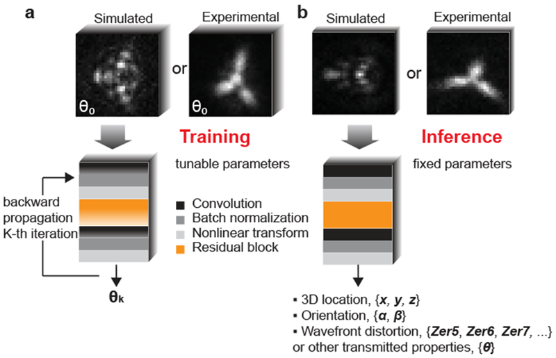
Figure 1:
Concept of training and inference with smNet and description of basic architecture.
( a ) smNet training process. The example input training data set consists of PSF images and the underlying true values of the measurements u03b8 0 . smNet takes in the training images and outputs est...
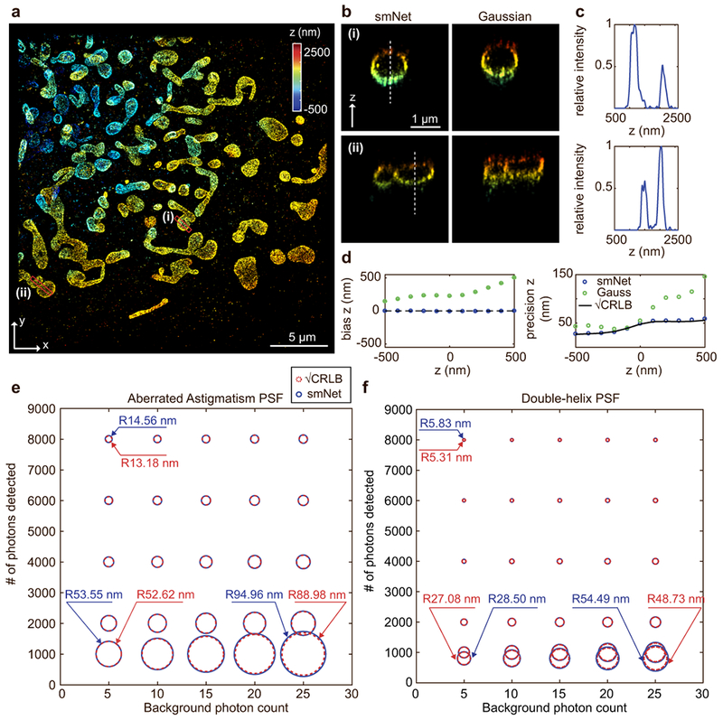
Figure 2:
3D-SMSN reconstruction using smNet and its error radii comparison with the CRLB for aberrated astigmatism and double helix PSFs.
( a ) 3D-SMSN reconstruction using smNet. The sample is TOM 20 in a COS-7 cell at a depth of 12 u00b5m from coverslip surface. Color represents the relative axial position of the localized molecules. ...
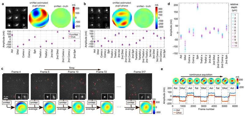
Figure 3:
smNet measures wavefront distortions.
( a,b ) smNet measurement of wavefront shape composed of 12 or 21 Zernike modes through simulated PSFs. The amplitude of each mode is randomly sampled from u2212159.15 to 159.15 mu03bb. The nine examp...
Figure images are served from the NIH/NLM PubMed Central Open Access Subset or Europe PMC; copyright remains with the publishers and authors.
💬 Discussion
0 commentsNo comments yet. Be the first to start a discussion!
Leave a Comment