Abstract
Electron microscopy (EM) facilitates analysis of the form, distribution, and functional status of key organelle systems in various pathological processes, including those associated with neurodegenerative disease. Such EM data often provide important new insights into the underlying disease mechanisms. The development of more accurate and efficient methods to quantify changes in subcellular microanatomy has already proven key to understanding the pathogenesis of Parkinson's and Alzheimer's diseases, as well as glaucoma. While our ability to acquire large volumes of 3D EM data is progressing rapidly, more advanced analysis tools are needed to assist in measuring precise three-dimensional morphologies of organelles within data sets that can include hundreds to thousands of whole cells. Although new imaging instrument throughputs can exceed teravoxels of data per day, image segmentation and analysis remain significant bottlenecks to achieving quantitative descriptions of whole cell structural organellomes. Here, we present a novel method for the automatic segmentation of organelles in 3D EM image stacks. Segmentations are generated using only 2D image information, making the method suitable for anisotropic imaging techniques such as serial block-face scanning electron microscopy (SBEM). Additionally, no assumptions about 3D organelle morphology are made, ensuring the method can be easily expanded to any number of structurally and functionally diverse organelles. Following the presentation of our algorithm, we validate its performance by assessing the segmentation accuracy of different organelle targets in an example SBEM dataset and demonstrate that it can be efficiently parallelized on supercomputing resources, resulting in a dramatic reduction in runtime.
🔬 Techniques
💻 Software
✨ Fluorophores
🧪 Sample Preparation
🔬 Cell Lines
🏭 Microscope Brands
💻 Software Details
🏛️ Research Organizations (ROR)
Affiliated research institutions:
📋 Methods
The description and validation of our method are arranged into three sections. In the first section, the workflow is described in detail. In the second, the robustness and accuracy of our method are validated by applying it to four different organelle targets (mitochondria, lysosomes, nuclei, and nucleoli) from a test SBEM dataset. In the third section, we describe experiments that demonstrate how our method can be easily scaled-up to accommodate the segmentation of teravoxel-sized datasets. The proposed method Image alignment and histogram specification All individual images of the input SBEM stack are converted to the MRC format and appended to an 8-bit MRC stack using the IMOD programs dm2mrc and newstack , respectively (Kremer et al., 1996 ). Sequential images within the stack are then translationally aligned to one another in the XY-plane using the cross-correlational alignment algorithm of the IMOD program tiltxcorr . To ensure consistency throughout the stack, the histograms of all images are matched to that of the first image in the stack using a MATLAB (The MathWorks, Inc., Natick, MA, U.S.A.) implementation of the exact histogram specification algorithm (Coltuc et al., 2006 ).
Generation of training images and labels
Once an organelle target has been selected by the experimenter, the next step is to generate a set of organelle-specific training images and labels to subsequently train a CHM pixel classifier. A set of N seed points, P, are selected throughout the processed SBEM stack in locations that possess at least one instance of the desired organelle, such that: P i = ( x i , y i , z i ) ∀ i ∈ { 1 , … , N } These points should be chosen in a manner that yields a wide distribution throughout the stack. After the selection of seed points, every instance of the chosen organelle is manually segmented in a Q × R pixel tile centered at each P i . Following manual segmentation, all tiles are extracted from the full SBEM stack using the IMOD program boxstartend . The extracted tiles will serve as training images, T i . Binary training labels, B i , are generated from each T i by applying the corresponding manual segmentation as a mask using the IMOD program imodmop . Thus, the final outputs from training data generation are (1) a stack of 8-bit, grayscale training images, T i , and (2) a stack of corresponding binary organelle masks, B i . Both stacks are of size Q × R × N. A flow chart illustrating this process is shown in Figure 2 . Figure 2 A flow chart of the steps involved in training data generation . The generation of a set of training data for mitochondrial automatic segmentation is shown here. First, a set of seed points, P i , are selected such that a wide distribution throughout the volume is achieved (bottom left). Tiles of size Q × R centered at each seed point are extracted to serve as training images, T i . All instances of the desired organelle target are manually segmented by a trained neuroanatomist on each training image. These manual segmentations are then used as masks to binarize each T i such that pixels of value one correspond to pixels of T i that are positive for the desired organelle. This process is repeated N times to yield stacks of training images and their corresponding training labels, B i . These stacks are then used to train a CHM classifier, C S,L , with the desired number of stages, S, and levels, L. Training organelle pixel classifiers with the cascaded hierarchical model The CHM consists of bottom-up and top-down steps cascaded in multiple stages (Seyedhosseini et al., 2013b ). The bottom-up step occurs in a user-specified number of hierarchical levels, L. At each level, the input stacks T i and B i are sequentially downsampled and a classifier is trained based on features extracted from the downsampled data as well as information from all lower levels of the hierarchy. After classifiers have been trained at all levels, the top-down path combines the coarse contextual information from higher levels into a single classifier that is applicable to images at native resolution. This whole process is then cascaded in a number of stages, S, where the output classifier from the previous stage serves as the input classifier for the subsequent stage. The final output is a pixel classifier, C S,L , that is applicable to images at the native pixel size of T i and B i . For optimal results, the number of stages chosen should be greater than one. The exact number of stages and levels chosen depends on a host of factors, including the size of T i and B i and the computational resources available to the experimenter.
Show full methods section
The description and validation of our method are arranged into three sections. In the first section, the workflow is described in detail. In the second, the robustness and accuracy of our method are validated by applying it to four different organelle targets (mitochondria, lysosomes, nuclei, and nucleoli) from a test SBEM dataset. In the third section, we describe experiments that demonstrate how our method can be easily scaled-up to accommodate the segmentation of teravoxel-sized datasets. The proposed method Image alignment and histogram specification All individual images of the input SBEM stack are converted to the MRC format and appended to an 8-bit MRC stack using the IMOD programs dm2mrc and newstack , respectively (Kremer et al., 1996 ). Sequential images within the stack are then translationally aligned to one another in the XY-plane using the cross-correlational alignment algorithm of the IMOD program tiltxcorr . To ensure consistency throughout the stack, the histograms of all images are matched to that of the first image in the stack using a MATLAB (The MathWorks, Inc., Natick, MA, U.S.A.) implementation of the exact histogram specification algorithm (Coltuc et al., 2006 ).
Generation of training images and labels
Once an organelle target has been selected by the experimenter, the next step is to generate a set of organelle-specific training images and labels to subsequently train a CHM pixel classifier. A set of N seed points, P, are selected throughout the processed SBEM stack in locations that possess at least one instance of the desired organelle, such that: P i = ( x i , y i , z i ) ∀ i ∈ { 1 , … , N } These points should be chosen in a manner that yields a wide distribution throughout the stack. After the selection of seed points, every instance of the chosen organelle is manually segmented in a Q × R pixel tile centered at each P i . Following manual segmentation, all tiles are extracted from the full SBEM stack using the IMOD program boxstartend . The extracted tiles will serve as training images, T i . Binary training labels, B i , are generated from each T i by applying the corresponding manual segmentation as a mask using the IMOD program imodmop . Thus, the final outputs from training data generation are (1) a stack of 8-bit, grayscale training images, T i , and (2) a stack of corresponding binary organelle masks, B i . Both stacks are of size Q × R × N. A flow chart illustrating this process is shown in Figure 2 . Figure 2 A flow chart of the steps involved in training data generation . The generation of a set of training data for mitochondrial automatic segmentation is shown here. First, a set of seed points, P i , are selected such that a wide distribution throughout the volume is achieved (bottom left). Tiles of size Q × R centered at each seed point are extracted to serve as training images, T i . All instances of the desired organelle target are manually segmented by a trained neuroanatomist on each training image. These manual segmentations are then used as masks to binarize each T i such that pixels of value one correspond to pixels of T i that are positive for the desired organelle. This process is repeated N times to yield stacks of training images and their corresponding training labels, B i . These stacks are then used to train a CHM classifier, C S,L , with the desired number of stages, S, and levels, L. Training organelle pixel classifiers with the cascaded hierarchical model The CHM consists of bottom-up and top-down steps cascaded in multiple stages (Seyedhosseini et al., 2013b ). The bottom-up step occurs in a user-specified number of hierarchical levels, L. At each level, the input stacks T i and B i are sequentially downsampled and a classifier is trained based on features extracted from the downsampled data as well as information from all lower levels of the hierarchy. After classifiers have been trained at all levels, the top-down path combines the coarse contextual information from higher levels into a single classifier that is applicable to images at native resolution. This whole process is then cascaded in a number of stages, S, where the output classifier from the previous stage serves as the input classifier for the subsequent stage. The final output is a pixel classifier, C S,L , that is applicable to images at the native pixel size of T i and B i . For optimal results, the number of stages chosen should be greater than one. The exact number of stages and levels chosen depends on a host of factors, including the size of T i and B i and the computational resources available to the experimenter.
Probability map generation
In the next step, a stack of test images, I j , are selected to apply the pixel classifier to. Depending on the goals of the experiment, these images may be full slices of the SBEM volume or extracted subvolumes. Prior to pixel classification, each I j is split into an m × n array of tiles such that the dimensions of each tile are roughly equivalent to the lateral dimensions of the training stacks, Q × R (step 3 of Algorithm 1 ). Tiling is performed with an overlap of U pixels between adjacent tiles. The choice of U is dependent on the size of the training stacks as well as the organelle target; in general, ideal values of U should fall in the range of 2–10% of Q and R. The previously generated CHM pixel classifier, C S,L , is then applied to each tile, yielding m × n probability map tiles (step 5 of Algorithm 1 ). All processed tiles are then stitched together to yield a final probability map, M j (step 7 of Algorithm 1 ). When stitching, the pixels in M j that correspond to regions of overlap between adjacent tiles are set to the maximum intensity pixel from all contributing tiles. Finally, M j is normalized such that each pixel ranges from [0, 1], with one representing the highest probability (step 8 of Algorithm 1 ). This process is then repeated over each I j to yield the final stack of probability maps. Algorithm 1 Organelle segmentation using tiled input images . 1: Declare values of m, n, U, G, α, and λ 2: for every test image I j do 3: Generate k = m × n tiles of I j with overlap U 4: for every k do 5: Apply the CHM classifier C S,L to the k-th tile 6: end for 7: Stitch all k tiles together to yield the probability map, M j 8: Normalize M j 9: Classify M j using Otsu's multi-level method with G gray levels, yielding O j 10: Threshold O j at the G-th level, giving the initial position mask K j 11: Perform morphological shrinking on K j 12: Segment M j by evolving active contours at initial positions specified by each unique 2D connected component of K j . Iterate α times with a smoothing factor of λ. The output is SEG j , the final segmentation of I j . 13: end for Binarization of probability maps Each probability map, M j , is binarized by evolving active contours (Chan and Vese, 2001 ) at automatically determined initial positions. For an unsupervised determination of the initial positions, the probability map M j is first thresholded using Otsu's multi-level method (Otsu, 1979 ) with G unique gray levels (step 9 of Algorithm 1 ). The output from this operation is O j , a map in which each pixel of M j has been classified into one of G unique levels, with the zeroth level corresponding to the approximate background. This map is then binarized by thresholding O j at a pixel intensity of G, yielding a mask of initial positions, K j (step 10 of Algorithm 1 ). This binary mask is then made smaller by applying two iterations of morphological shrinking (step 11 of Algorithm 1 ) and used to initialize the evolution of active contours with a number of iterations and smoothing factor specified by α and λ, respectively (step 12 of Algorithm 1 ). Each 2D connected component of K j serves as a unique initial position for contour evolution. For best results, α should be at least 50. The choice of λ depends largely on the organelle target and pixel size of the test images, but in general should fall in the range of 0–8. Larger values of λ can be used when the pixel size is small. If the pixel size is too large (i.e., above 10 nm/pixel), smoothing should be turned off by setting λ to zero. The value of G significantly alters the results, and its choice is dependent on the goals of the experimenter. Low values of G tend to emphasize true positives at the risk of retaining false positives. As G is increased, false positives are more readily removed, but so are true positives. The final output from this process is SEG j , the organelle segmentation of the input grayscale image, I j . An illustration of this process is shown for two test images in Figure 3 . Figure 3 The binarization of probability maps using active contours initialized by a multi-level Otsu threshold yields accurate segmentation results . Colorized maps, M, of a nucleus (A) and lysosomes (D) generated by applying Otsu's method with multiple levels to probability maps obtained by CHM pixel classification. Each color corresponds to a unique level of the threshold. Six gray levels ( G = 6) were used for the nucleus and four ( G = 4) were used for the lysosomes. Initial positions (B,E) were determined by selecting pixels corresponding to only the highest levels of each threshold followed by two iterations of morphological shrinking. Output segmentations (C,F) were obtained by evolving active contours about each of the initial positions in (B,E) with 100 iterations and a smoothing factor of 8 (α = 100, λ = 8). In the case of the lysosome images, note that a myelinated axon that was originally detected by the classifier as a false positive ( D , arrow) has been removed from the final segmentation by the application of our method ( F , arrow). Meshing Each output SEG j is converted to the MRC format and appended to an MRC stack. Contours are drawn around each 2D connected component using the IMOD program imodauto . The output contours are then three-dimensionally meshed together using the program imodmesh , and separate 3D connected components are sorted into different objects using the program imodsortsurf . Meshing is performed using the low resolution option to reduce the effect of translational artifacts between subsequent image slices.
Experimental validation
Tissue processing, image acquisition, and preprocessing The suprachiasmatic nucleus (SCN) of one 3-month-old, male C57BL/6J mouse was harvested and prepared for SBEM using a standard protocol (Wilke et al., 2013 ). The resin-embedded tissue was mounted on an aluminum specimen pin and prepared for SBEM imaging as previously described (Holcomb et al., 2013 ). Imaging was performed by detection of backscattered electrons (BSE) using a Zeiss Merlin scanning electron microscope equipped with a 3View ultramicrotome (Gatan). The SBEM image stack was acquired in ultrahigh vacuum mode using an accelerating voltage of 1.9 kV, a pixel dwell time of 500 ns, and a spot size of 1.0. Sectioning was performed with a cutting thickness of 30 nm. BSE images were acquired at 800x magnification with a raster size of 32,000 pixels × 24,000 pixels, yielding a pixel size of 3.899 nm/pixel. A total of 1283 serial images were acquired, resulting in an image stack with tissue dimensions of roughly 124.8 × 93.6 × 38.5 μm (~450,000 μm 3 ). The specimen was then removed from the chamber, and an image of a diffraction grating replica specimen (Ted Pella, Redding, CA, U.S.A.) was acquired for calibration of the lateral pixel size. Low magnification images of the block-face were acquired before and after sectioning. Image alignment was performed as described in Section Image Alignment and Histogram Specification. Following alignment, the stack was downsampled in the XY-plane by a factor of two, yielding a final stack with pixel dimensions of 16,000 × 12,000 × 1283 and pixel sizes of 7.799 nm/pixel and 30 nm/pixel in the lateral and axial dimensions, respectively. Since preliminary results did not demonstrate noticeable differences in the output of our method between the native resolution stack and the downsampled stack, downsampling was performed to reduce processing time. Exact histogram specification was performed as previously described. All image alignment and pre-processing steps were performed on a custom workstation (Advanced HPC, San Diego, CA, U.S.A.) with the following configuration: Xeon X5690 3.47 GHZ CPU, 48 GB RAM, 32 TB HDD, NVIDIA Quadro FX 3800, CentOS release 6.2.
Automatic segmentation
The four types of organelles targeted for automatic segmentation were mitochondria, lysosomes, nuclei, and nucleoli. These targets were chosen because they are morphologically and texturally diverse, and thus pose a significant test of the robustness of our method. For each organelle target, 90 seed points were placed throughout the SBEM stack as described in Section Generation of Training Images and Labels. Training data and labels were created using the values shown in Table 1 . Of the 90 tiles generated for each organelle, 50 were randomly selected for use in training a CHM classifier; the other 40 were set aside to use as test data for validation. Organelle-specific CHM classifiers were trained using the values shown in Table 1 . The performances of all classifiers were evaluated by preparing receiver operating characteristic (ROC) curves (Fawcett, 2006 ). Each classifier was then used to generate probability maps of the 40 test images corresponding to its organelle. Segmentation was performed as described in Section Binarization of Probability Maps using the values shown in Table 1 . All training, pixel classification, and segmentation steps were performed on the National Biomedical Computation Resource (NBCR) cluster, rocce.ucsd.edu ( http://rocce-mgr.ucsd.edu/ ). Table 1 Parameter sets used for the validation of specific organelle targets . Parameter Variable Mitochondria Lysosomes Nuclei Nucleoli Number of training slices N 50 50 50 50 Lateral dimensions of each training slice Q, R 500, 500 500, 500 500, 500 500, 500 Number of CHM levels L 2 2 2 2 Number of CHM stages S 2 2 2 2 Size of tile array m, n 2, 2 2, 2 2, 2 2, 2 Tiling overlap U 50 50 20 50 Gray levels for multi-level Otsu thresholding G 3 2 2 2 Active contour iterations α 80 200 300 90 Smoothing factor λ 7 4 8 10 Validation of the active contour segmentation of CHM probability maps Evaluation metrics were computed for each set of organelle-specific test images by comparing their segmentations with manually segmented ground truth. For each stack, the confusion matrix consisting of the number of true positive (TP), false positive (FP), true negative (TN), and false negative (FN) pixels was computed and used to calculate the true positive rate (TPR), false positive rate (FPR), precision, accuracy, and F -value, such that: TPR = TP TP+FN FPR = FP FP+TN Precision = TP TP+FP Accuracy = TP+TN TP+FN+FP+TN F-value = 2 × Precision × TPR Precision+TPR This analysis was then repeated with segmentations generated from the same probability maps, but with a number of different unsupervised binarization algorithms: (1) Minimum error thresholding (Kittler and Illingworth, 1986 ), (2) Maximum entropy thresholding (Kapur et al., 1985 ), and (3) Otsu's single-level method (Otsu, 1979 ). The performance of each algorithm, as quantified with the above metrics, was compared against that of our own method for each organelle target. Since ground truth was available, the pixel intensity threshold that maximized the F -value of each probability map with respect to its corresponding ground truth was determined by computing the F -value at incrementally increasing thresholds from [0, …, 1] and taking the maximum value.
Scale-up to teravoxel-sized datasets
Determination of optimal downsampling levels for different organelles
Since the segmentation of entire SBEM datasets is computationally intensive, we first decided to determine to what degree input images could be downsampled before segmentation results were adversely affected. Downsampled versions of each set of training images, training labels, and test images were prepared for all four organelle targets. Downsampling was performed by factors of two, three, four, and five, yielding pixel sizes of roughly 15.59, 23.39, 31.19, and 38.90 nm/pixel, respectively. CHM classifiers with two stages and two levels were trained for each set of downsampled, organelle-specific training images and labels. Probability maps were computed with m = 2, n = 2, and U = 20. Segmentations were generated using the active contour method with G = 2, α = 100, and λ = 0. For each set of output segmentations, evaluation metrics were computed as described in Section Validation of the Active Contour Segmentation of CHM Probability Maps.
Segmentation of organelles from a full SBEM stack
The entire test dataset was laterally downsampled by a factor of eight, yielding a final stack with dimensions of 4000 × 3000 × 1283 pixels. The corresponding CHM classifiers generated in Section Determination of Optimal Downsampling Levels for Different Organelles were applied to produce stacks of probability maps at this pixel size for nuclei, nucleoli, and mitochondria. Processing was performed using an 8 × 6 tile array with an overlap of 20 pixels between adjacent tiles. Tiling, pixel classification, stitching, and binarization were performed using one CPU for each input image. One hundred total CPUs were used, such that 100 images were processed in parallel to expedite processing. All steps were performed on the National Biomedical Computation Resource (NBCR) cluster, rocce.ucsd.edu. Following probability map generation, all images were appended to organelle-specific MRC stacks, and contours and surface renderings were generated as described in Section Meshing.
Comparison to a previously published algorithm
The results of our approach to nuclear automatic segmentation were validated by comparison with the results obtained by the algorithm of Tek et al. ( 2014 ). The full dataset was first downsampled to isotropic voxel dimensions (30 × 30 × 30 nm), resulting in a stack of size 4029 × 3120 × 1283 voxels. Training data and images consisted of a 500 × 500 × 50 subvolume of the downsampled stack containing two adjacent nuclei. Ground truth data were generated by manual segmentation of all neuronal, glial, and endothelial cell nuclei across fifty consecutive slices from the center of the dataset. A CHM pixel classifier with two stages and two levels was trained and applied to all images in the stack. Similarly, an ilastik voxel classifier was trained using all possible features with the same training images serving as input (Sommer et al., 2011 ). This classifier was subsequently applied to all images in the downsampled stack. CHM probability maps were binarized using the proposed method. The ilastik probability maps were binarized by thresholding at the level p = 0.5, followed by the application of the object detection algorithm of Tek and colleagues with V th1 and V th2 set to 25 and 10,000, respectively (Tek et al., 2014 ). The source code for CHM and all related scripts are available to download from http://www.sci.utah.edu/software/chm.html . The training images, training labels, and test images used in this study have also been made available to download at this URL.
The proposed method Image alignment and histogram specification All individual images of the input SBEM stack are converted to the MRC format and appended to an 8-bit MRC stack using the IMOD programs dm2mrc and newstack , respectively (Kremer et al., 1996 ). Sequential images within the stack are then translationally aligned to one another in the XY-plane using the cross-correlational alignment algorithm of the IMOD program tiltxcorr . To ensure consistency throughout the stack, the histograms of all images are matched to that of the first image in the stack using a MATLAB (The MathWorks, Inc., Natick, MA, U.S.A.) implementation of the exact histogram specification algorithm (Coltuc et al., 2006 ).
Generation of training images and labels
Once an organelle target has been selected by the experimenter, the next step is to generate a set of organelle-specific training images and labels to subsequently train a CHM pixel classifier. A set of N seed points, P, are selected throughout the processed SBEM stack in locations that possess at least one instance of the desired organelle, such that: P i = ( x i , y i , z i ) ∀ i ∈ { 1 , … , N } These points should be chosen in a manner that yields a wide distribution throughout the stack. After the selection of seed points, every instance of the chosen organelle is manually segmented in a Q × R pixel tile centered at each P i . Following manual segmentation, all tiles are extracted from the full SBEM stack using the IMOD program boxstartend . The extracted tiles will serve as training images, T i . Binary training labels, B i , are generated from each T i by applying the corresponding manual segmentation as a mask using the IMOD program imodmop . Thus, the final outputs from training data generation are (1) a stack of 8-bit, grayscale training images, T i , and (2) a stack of corresponding binary organelle masks, B i . Both stacks are of size Q × R × N. A flow chart illustrating this process is shown in Figure 2 . Figure 2 A flow chart of the steps involved in training data generation . The generation of a set of training data for mitochondrial automatic segmentation is shown here. First, a set of seed points, P i , are selected such that a wide distribution throughout the volume is achieved (bottom left). Tiles of size Q × R centered at each seed point are extracted to serve as training images, T i . All instances of the desired organelle target are manually segmented by a trained neuroanatomist on each training image. These manual segmentations are then used as masks to binarize each T i such that pixels of value one correspond to pixels of T i that are positive for the desired organelle. This process is repeated N times to yield stacks of training images and their corresponding training labels, B i . These stacks are then used to train a CHM classifier, C S,L , with the desired number of stages, S, and levels, L. Training organelle pixel classifiers with the cascaded hierarchical model The CHM consists of bottom-up and top-down steps cascaded in multiple stages (Seyedhosseini et al., 2013b ). The bottom-up step occurs in a user-specified number of hierarchical levels, L. At each level, the input stacks T i and B i are sequentially downsampled and a classifier is trained based on features extracted from the downsampled data as well as information from all lower levels of the hierarchy. After classifiers have been trained at all levels, the top-down path combines the coarse contextual information from higher levels into a single classifier that is applicable to images at native resolution. This whole process is then cascaded in a number of stages, S, where the output classifier from the previous stage serves as the input classifier for the subsequent stage. The final output is a pixel classifier, C S,L , that is applicable to images at the native pixel size of T i and B i . For optimal results, the number of stages chosen should be greater than one. The exact number of stages and levels chosen depends on a host of factors, including the size of T i and B i and the computational resources available to the experimenter.
Probability map generation
In the next step, a stack of test images, I j , are selected to apply the pixel classifier to. Depending on the goals of the experiment, these images may be full slices of the SBEM volume or extracted subvolumes. Prior to pixel classification, each I j is split into an m × n array of tiles such that the dimensions of each tile are roughly equivalent to the lateral dimensions of the training stacks, Q × R (step 3 of Algorithm 1 ). Tiling is performed with an overlap of U pixels between adjacent tiles. The choice of U is dependent on the size of the training stacks as well as the organelle target; in general, ideal values of U should fall in the range of 2–10% of Q and R. The previously generated CHM pixel classifier, C S,L , is then applied to each tile, yielding m × n probability map tiles (step 5 of Algorithm 1 ). All processed tiles are then stitched together to yield a final probability map, M j (step 7 of Algorithm 1 ). When stitching, the pixels in M j that correspond to regions of overlap between adjacent tiles are set to the maximum intensity pixel from all contributing tiles. Finally, M j is normalized such that each pixel ranges from [0, 1], with one representing the highest probability (step 8 of Algorithm 1 ). This process is then repeated over each I j to yield the final stack of probability maps. Algorithm 1 Organelle segmentation using tiled input images . 1: Declare values of m, n, U, G, α, and λ 2: for every test image I j do 3: Generate k = m × n tiles of I j with overlap U 4: for every k do 5: Apply the CHM classifier C S,L to the k-th tile 6: end for 7: Stitch all k tiles together to yield the probability map, M j 8: Normalize M j 9: Classify M j using Otsu's multi-level method with G gray levels, yielding O j 10: Threshold O j at the G-th level, giving the initial position mask K j 11: Perform morphological shrinking on K j 12: Segment M j by evolving active contours at initial positions specified by each unique 2D connected component of K j . Iterate α times with a smoothing factor of λ. The output is SEG j , the final segmentation of I j . 13: end for Binarization of probability maps Each probability map, M j , is binarized by evolving active contours (Chan and Vese, 2001 ) at automatically determined initial positions. For an unsupervised determination of the initial positions, the probability map M j is first thresholded using Otsu's multi-level method (Otsu, 1979 ) with G unique gray levels (step 9 of Algorithm 1 ). The output from this operation is O j , a map in which each pixel of M j has been classified into one of G unique levels, with the zeroth level corresponding to the approximate background. This map is then binarized by thresholding O j at a pixel intensity of G, yielding a mask of initial positions, K j (step 10 of Algorithm 1 ). This binary mask is then made smaller by applying two iterations of morphological shrinking (step 11 of Algorithm 1 ) and used to initialize the evolution of active contours with a number of iterations and smoothing factor specified by α and λ, respectively (step 12 of Algorithm 1 ). Each 2D connected component of K j serves as a unique initial position for contour evolution. For best results, α should be at least 50. The choice of λ depends largely on the organelle target and pixel size of the test images, but in general should fall in the range of 0–8. Larger values of λ can be used when the pixel size is small. If the pixel size is too large (i.e., above 10 nm/pixel), smoothing should be turned off by setting λ to zero. The value of G significantly alters the results, and its choice is dependent on the goals of the experimenter. Low values of G tend to emphasize true positives at the risk of retaining false positives. As G is increased, false positives are more readily removed, but so are true positives. The final output from this process is SEG j , the organelle segmentation of the input grayscale image, I j . An illustration of this process is shown for two test images in Figure 3 . Figure 3 The binarization of probability maps using active contours initialized by a multi-level Otsu threshold yields accurate segmentation results . Colorized maps, M, of a nucleus (A) and lysosomes (D) generated by applying Otsu's method with multiple levels to probability maps obtained by CHM pixel classification. Each color corresponds to a unique level of the threshold. Six gray levels ( G = 6) were used for the nucleus and four ( G = 4) were used for the lysosomes. Initial positions (B,E) were determined by selecting pixels corresponding to only the highest levels of each threshold followed by two iterations of morphological shrinking. Output segmentations (C,F) were obtained by evolving active contours about each of the initial positions in (B,E) with 100 iterations and a smoothing factor of 8 (α = 100, λ = 8). In the case of the lysosome images, note that a myelinated axon that was originally detected by the classifier as a false positive ( D , arrow) has been removed from the final segmentation by the application of our method ( F , arrow). Meshing Each output SEG j is converted to the MRC format and appended to an MRC stack. Contours are drawn around each 2D connected component using the IMOD program imodauto . The output contours are then three-dimensionally meshed together using the program imodmesh , and separate 3D connected components are sorted into different objects using the program imodsortsurf . Meshing is performed using the low resolution option to reduce the effect of translational artifacts between subsequent image slices.
Experimental validation
Tissue processing, image acquisition, and preprocessing The suprachiasmatic nucleus (SCN) of one 3-month-old, male C57BL/6J mouse was harvested and prepared for SBEM using a standard protocol (Wilke et al., 2013 ). The resin-embedded tissue was mounted on an aluminum specimen pin and prepared for SBEM imaging as previously described (Holcomb et al., 2013 ). Imaging was performed by detection of backscattered electrons (BSE) using a Zeiss Merlin scanning electron microscope equipped with a 3View ultramicrotome (Gatan). The SBEM image stack was acquired in ultrahigh vacuum mode using an accelerating voltage of 1.9 kV, a pixel dwell time of 500 ns, and a spot size of 1.0. Sectioning was performed with a cutting thickness of 30 nm. BSE images were acquired at 800x magnification with a raster size of 32,000 pixels × 24,000 pixels, yielding a pixel size of 3.899 nm/pixel. A total of 1283 serial images were acquired, resulting in an image stack with tissue dimensions of roughly 124.8 × 93.6 × 38.5 μm (~450,000 μm 3 ). The specimen was then removed from the chamber, and an image of a diffraction grating replica specimen (Ted Pella, Redding, CA, U.S.A.) was acquired for calibration of the lateral pixel size. Low magnification images of the block-face were acquired before and after sectioning. Image alignment was performed as described in Section Image Alignment and Histogram Specification. Following alignment, the stack was downsampled in the XY-plane by a factor of two, yielding a final stack with pixel dimensions of 16,000 × 12,000 × 1283 and pixel sizes of 7.799 nm/pixel and 30 nm/pixel in the lateral and axial dimensions, respectively. Since preliminary results did not demonstrate noticeable differences in the output of our method between the native resolution stack and the downsampled stack, downsampling was performed to reduce processing time. Exact histogram specification was performed as previously described. All image alignment and pre-processing steps were performed on a custom workstation (Advanced HPC, San Diego, CA, U.S.A.) with the following configuration: Xeon X5690 3.47 GHZ CPU, 48 GB RAM, 32 TB HDD, NVIDIA Quadro FX 3800, CentOS release 6.2.
Automatic segmentation
The four types of organelles targeted for automatic segmentation were mitochondria, lysosomes, nuclei, and nucleoli. These targets were chosen because they are morphologically and texturally diverse, and thus pose a significant test of the robustness of our method. For each organelle target, 90 seed points were placed throughout the SBEM stack as described in Section Generation of Training Images and Labels. Training data and labels were created using the values shown in Table 1 . Of the 90 tiles generated for each organelle, 50 were randomly selected for use in training a CHM classifier; the other 40 were set aside to use as test data for validation. Organelle-specific CHM classifiers were trained using the values shown in Table 1 . The performances of all classifiers were evaluated by preparing receiver operating characteristic (ROC) curves (Fawcett, 2006 ). Each classifier was then used to generate probability maps of the 40 test images corresponding to its organelle. Segmentation was performed as described in Section Binarization of Probability Maps using the values shown in Table 1 . All training, pixel classification, and segmentation steps were performed on the National Biomedical Computation Resource (NBCR) cluster, rocce.ucsd.edu ( http://rocce-mgr.ucsd.edu/ ). Table 1 Parameter sets used for the validation of specific organelle targets . Parameter Variable Mitochondria Lysosomes Nuclei Nucleoli Number of training slices N 50 50 50 50 Lateral dimensions of each training slice Q, R 500, 500 500, 500 500, 500 500, 500 Number of CHM levels L 2 2 2 2 Number of CHM stages S 2 2 2 2 Size of tile array m, n 2, 2 2, 2 2, 2 2, 2 Tiling overlap U 50 50 20 50 Gray levels for multi-level Otsu thresholding G 3 2 2 2 Active contour iterations α 80 200 300 90 Smoothing factor λ 7 4 8 10 Validation of the active contour segmentation of CHM probability maps Evaluation metrics were computed for each set of organelle-specific test images by comparing their segmentations with manually segmented ground truth. For each stack, the confusion matrix consisting of the number of true positive (TP), false positive (FP), true negative (TN), and false negative (FN) pixels was computed and used to calculate the true positive rate (TPR), false positive rate (FPR), precision, accuracy, and F -value, such that: TPR = TP TP+FN FPR = FP FP+TN Precision = TP TP+FP Accuracy = TP+TN TP+FN+FP+TN F-value = 2 × Precision × TPR Precision+TPR This analysis was then repeated with segmentations generated from the same probability maps, but with a number of different unsupervised binarization algorithms: (1) Minimum error thresholding (Kittler and Illingworth, 1986 ), (2) Maximum entropy thresholding (Kapur et al., 1985 ), and (3) Otsu's single-level method (Otsu, 1979 ). The performance of each algorithm, as quantified with the above metrics, was compared against that of our own method for each organelle target. Since ground truth was available, the pixel intensity threshold that maximized the F -value of each probability map with respect to its corresponding ground truth was determined by computing the F -value at incrementally increasing thresholds from [0, …, 1] and taking the maximum value.
📊 Figures
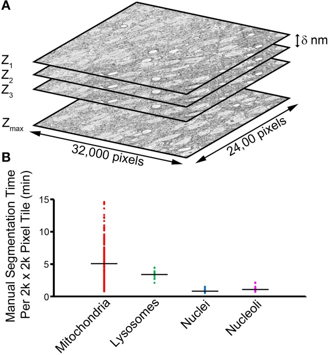
Figure 1
The manual segmentation of organelles from SBEM image stacks represents a significant bottleneck to quantitative analyses . (A) A typical SBEM dataset consists of individual image slices collected in ...
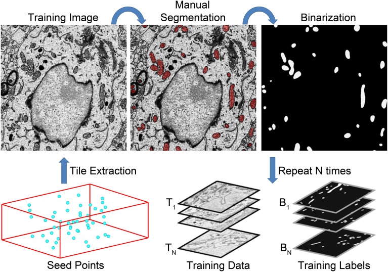
Figure 2
A flow chart of the steps involved in training data generation . The generation of a set of training data for mitochondrial automatic segmentation is shown here. First, a set of seed points, P i , are...
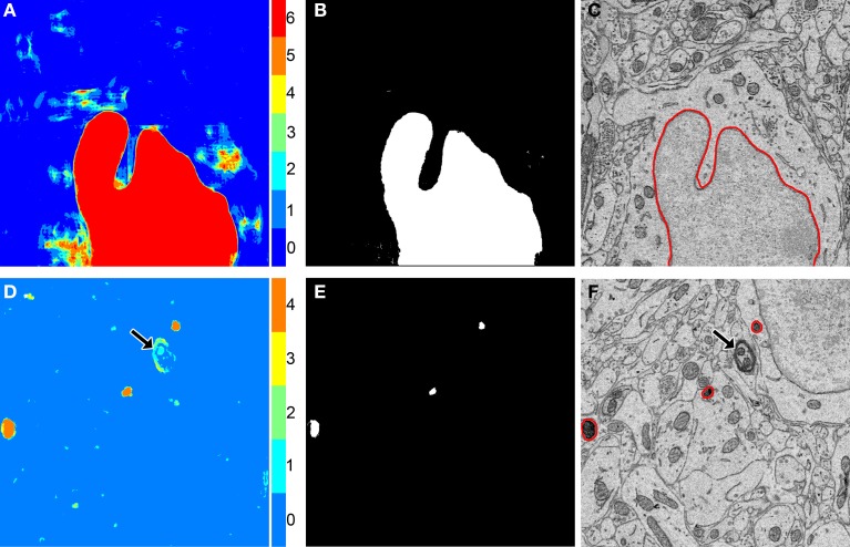
Figure 3
The binarization of probability maps using active contours initialized by a multi-level Otsu threshold yields accurate segmentation results . Colorized maps, M, of a nucleus (A) and lysosomes (D) gene...
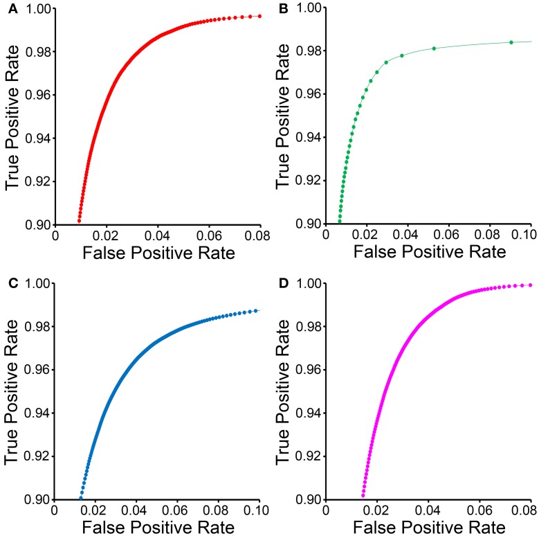
Figure 4
ROC curves for CHM classifiers of various organelles . ROC curves for mitochondrial (A) , lysosomal (B) , nuclear (C) , and nucleolar (D) CHM classifiers generated with two stages and two levels.
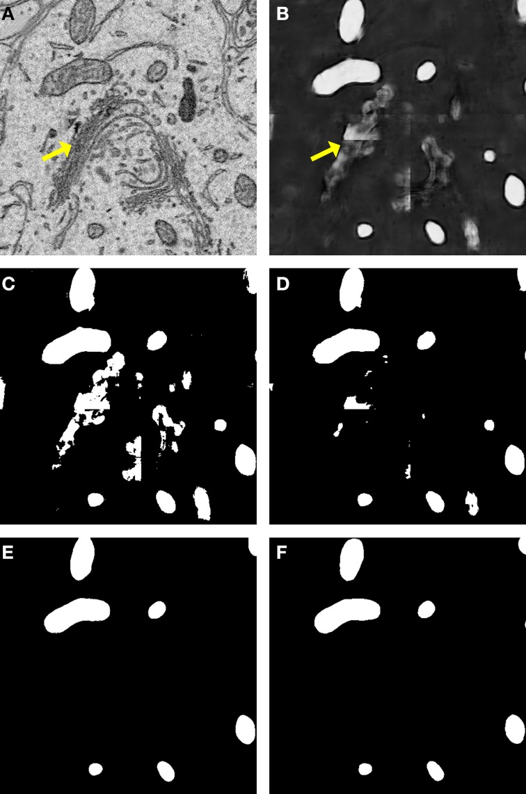
Figure 5
Binarization of probability maps using active contours outperforms other methods . A CHM classifier for mitochondria was applied to a 500 u00d7 500 pixel test image (A) , generating the probability ma...
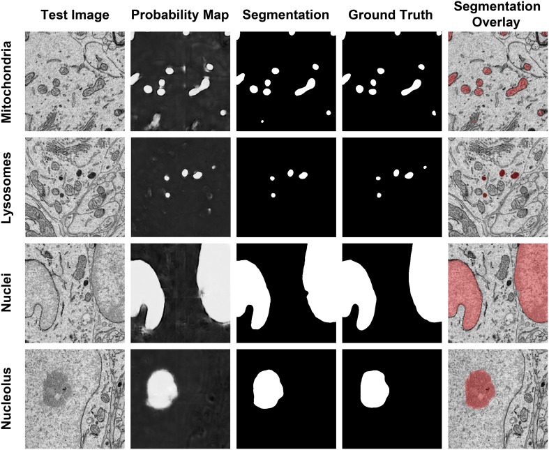
Figure 6
The results of our method are consistent when applied to diverse organelle targets . The application of our method to different organelle targets yields consistent results without the need to signific...
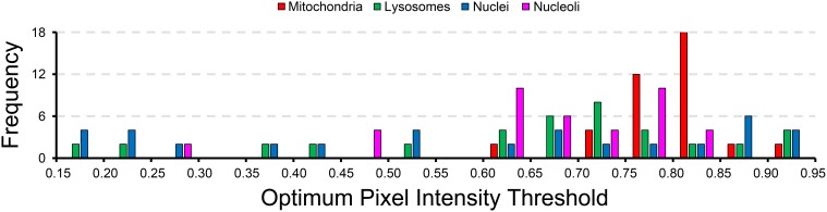
Figure 7
The wide distribution of optimum pixel intensity thresholds demonstrates the usefulness of our method for probability map binarization . The probability map pixel intensity threshold that maximized th...
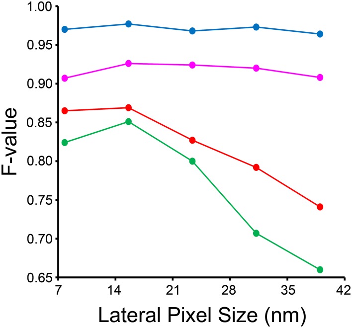
Figure 8
Input images can be downsampled to various degrees before the segmentation results are negatively affected . Each organelle-specific stack was downsampled by factors of two, four, six, eight, and ten....
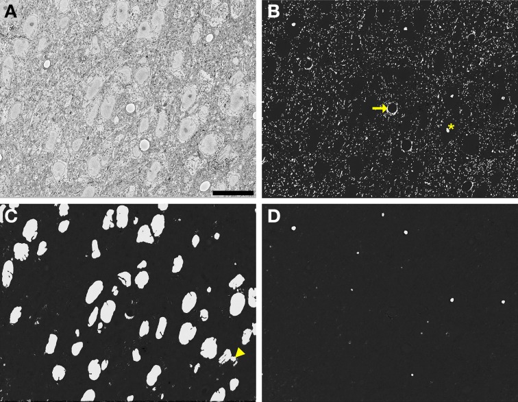
Figure 9
Automatic segmentation can be efficiently scaled to handle full slices from teravoxel-sized SBEM datasets . Probability maps of full images from the SCN dataset were generated by downsampling the imag...
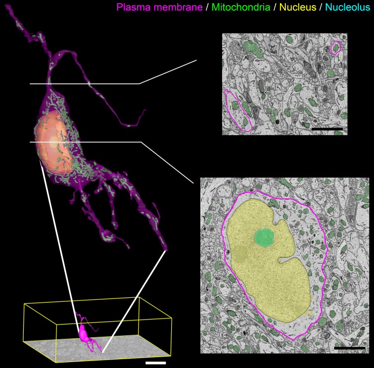
Figure 10
Output surface renderings of manually segmented organelles within an SCN neuron . The plasma membrane of a neuron was manually traced in its entirety throughout the dataset. The size of this neuron wi...
Figure images are served from the NIH/NLM PubMed Central Open Access Subset or Europe PMC; copyright remains with the publishers and authors.
💬 Discussion
0 commentsNo comments yet. Be the first to start a discussion!
Leave a Comment