Abstract
Neural integrators are involved in a variety of sensorimotor and cognitive behaviors. The oculomotor system contains a simple example, a hindbrain neural circuit that takes velocity signals as inputs and temporally integrates them to control eye position. Here we investigated the structural underpinnings of temporal integration in the larval zebrafish by first identifying integrator neurons using two-photon calcium imaging and then reconstructing the same neurons through serial electron microscopic analysis. Integrator neurons were identified as those neurons with activities highly correlated with eye position during spontaneous eye movements. Three morphological classes of neurons were observed: ipsilaterally projecting neurons located medially, contralaterally projecting neurons located more laterally, and a population at the extreme lateral edge of the hindbrain for which we were not able to identify axons. Based on their somatic locations, we inferred that neurons with only ipsilaterally projecting axons are glutamatergic, whereas neurons with only contralaterally projecting axons are largely GABAergic. Dendritic and synaptic organization of the ipsilaterally projecting neurons suggests a broad sampling from inputs on the ipsilateral side. We also observed the first conclusive evidence of synapses between integrator neurons, which have long been hypothesized by recurrent network models of integration via positive feedback.
🔬 Techniques
✨ Fluorophores
🧪 Sample Preparation
🏭 Microscope Brands
🧪 Reagent Suppliers
💻 Software Details
🏛️ Research Organizations (ROR)
Affiliated research institutions:
📋 Methods
Text Contact for reagent and resource sharing
For further information regarding the any resources and reagents please contact ashwinv@princeton.edu .
Experimental model and subject details
All zebrafish larvae experimental procedures were approved by Weill Cornell Medical College’s Institutional Animal Care and Use Committee. We used nacre mutant zebrafish larva, 6 days of age for all experiments.
Method details Two-photon calcium imaging
A nacre mutant zebrafish larva, 6 days of age, was anesthetized in 100 mg/L tricaine-methanesulfonate (MS222, VWR TCT0941- 025G) for about 1 minute and then quickly mounted dorsal side up with droplets of 1.7% low temperature agarose (Sigma A0701-100G) on the lid of a 35mm petri dish containing a bed of hardened 1% agarose (Invitrogen 15510-027). The larva was then covered in 50 mg/L MS222. The larva was bulk-loaded [ 46 , 47 ] with calcium sensitive dye Oregon Green 488 BAPTA-1 AM (5 mM, in DMSO with 5% pluronic, Invitrogen, O-6807) by inserting a capillary through the dorsal skin surface over the lateral edge of the right side of the hindbrain just caudal to the cerebellum, at ~30° decline relative to the dorsal surface. Following recovery, hindbrain of the animal was imaged at 790nm on predefined planes at 1 Hz. The imaging was performed unilaterally on three pre-defined planes ~ 8μm apart, below the level of the Mauthner neuron. The integrator neurons were identified in a manner similar to a previously described method [ 48 , 49 ]. Briefly, correlations for every pixel over a 5 min acquisition period was determined for eye position and eye velocity. A region-of-Interest (ROI) was then drawn over the pixels where the majority were correlated to one of these variables. The fluorescence was reported as change in fluorescence for each frame relative to the average fluorescence, divided by the average. Saccadic fluorescence traces were displayed over an 8 sec window starting 1 sec before the end of the saccade. The firing rates were computed over a 6 second fixation period beginning 1 sec after the end of the saccade. The firing rates were computed by deconvolving the average fluorescent traces with a calcium impulse response function (CIRF) as described previously [ 30 ]. The integrator time constants were calculated by fitting an exponential function (Matlab ezfit) to to the firing rates. The time constants for the fits were capped at 100 sec.
Show full methods section
Text Contact for reagent and resource sharing
For further information regarding the any resources and reagents please contact ashwinv@princeton.edu .
Experimental model and subject details
All zebrafish larvae experimental procedures were approved by Weill Cornell Medical College’s Institutional Animal Care and Use Committee. We used nacre mutant zebrafish larva, 6 days of age for all experiments.
Method details Two-photon calcium imaging
A nacre mutant zebrafish larva, 6 days of age, was anesthetized in 100 mg/L tricaine-methanesulfonate (MS222, VWR TCT0941- 025G) for about 1 minute and then quickly mounted dorsal side up with droplets of 1.7% low temperature agarose (Sigma A0701-100G) on the lid of a 35mm petri dish containing a bed of hardened 1% agarose (Invitrogen 15510-027). The larva was then covered in 50 mg/L MS222. The larva was bulk-loaded [ 46 , 47 ] with calcium sensitive dye Oregon Green 488 BAPTA-1 AM (5 mM, in DMSO with 5% pluronic, Invitrogen, O-6807) by inserting a capillary through the dorsal skin surface over the lateral edge of the right side of the hindbrain just caudal to the cerebellum, at ~30° decline relative to the dorsal surface. Following recovery, hindbrain of the animal was imaged at 790nm on predefined planes at 1 Hz. The imaging was performed unilaterally on three pre-defined planes ~ 8μm apart, below the level of the Mauthner neuron. The integrator neurons were identified in a manner similar to a previously described method [ 48 , 49 ]. Briefly, correlations for every pixel over a 5 min acquisition period was determined for eye position and eye velocity. A region-of-Interest (ROI) was then drawn over the pixels where the majority were correlated to one of these variables. The fluorescence was reported as change in fluorescence for each frame relative to the average fluorescence, divided by the average. Saccadic fluorescence traces were displayed over an 8 sec window starting 1 sec before the end of the saccade. The firing rates were computed over a 6 second fixation period beginning 1 sec after the end of the saccade. The firing rates were computed by deconvolving the average fluorescent traces with a calcium impulse response function (CIRF) as described previously [ 30 ]. The integrator time constants were calculated by fitting an exponential function (Matlab ezfit) to to the firing rates. The time constants for the fits were capped at 100 sec.
Serial section electron microscopy
The animal was immersed in a fixative mixture of 2% paraformaldehyde and 2.25% glutaraldehyde buffered in 65 mM cacodylate buffer. The skin over the hindbrain was removed for good ultrastructure preservation and homogeneous staining of the tissue. Then it was thoroughly washed in 0.1M cacodylate buffer with 4% sucrose before staining. The tissue was stained using a conventional ROTO procedure [ 50 ]. Briefly, the specimen was stained in 1% reduced osmium tetroxide with potassium ferrocyanide for 2 hr on ice. The tissue was then washed 4x 30 min in 0.1M cacodylate buffer, also on ice. This was then followed by amplification in 1% sodium thiocarbohydroazide (TCH) for 15 min followed by 3×5 min washes in water and another round of incubation in 1% osmium tetroxide for 1 hr. The tissue was then washed 3×15 min in water and incubated with 1% aqueous uranyl acetate overnight. The following day the tissue was washed 3×15 min in water and incubated for 30 min in Lead aspartate solution, followed by washing and dehydration with a series of ethanol washes, followed by propylene oxide (PO) washes. The tissue was then infiltrated in decreasing gradients of PO and EPON for 24 hrs and baked for 48 hrs at 60 C. Following hardening, the tissue block face was coarsely trimmed and a rectangular mesa was defined for serial sectioning. Care was taken to orient the specimen to permit sectioning along the horizontal axis. Serial sections from the above animal were collected approximately from the level of the Mauthner axon at a thickness of 45 nm. The serial sections were then adhered to a silicon wafer, using double sided carbon tape (TEDpella), the wafers were coated with a thin film of carbon to make them conductive. The serial sections were collected using the automatic tape-collecting ultramicrotome (ATUM) [ 51 , 52 ]. Each wafer was imaged in a Zeiss Sigma field emitting scanning electron microscope in the backscattered electron mode using a custom software interface to collected the images [ 51 ]. For the high-resolution each section was imaged at a lateral resolution of 5nm/pixel in a region of interest that roughly corresponded with the area imaged on the light microscopic. The EM volume we imaged contained 15791 image tiles (8000×8000 pixels each) or ~ 10 11 pixels. The imaged volume was 220×112×57μm 3 (RC X ML X DV). Registration of light microscope and electron microscope volumes The EM images were aligned using the TrakEM2 plugin in Fiji [ 53 ]. Briefly, individual images were imported into the TrakEM2 framework and montaged using affine and elastic transforms. The images were then registered in z using a similar approach, where the first pass was performed using affine transforms, followed by elastic transforms. All the alignment was performed on a machine with 32 virtual cores and 120GB RAM. To locate the cells that were involved in the integrator circuit, we first made use of the fact that gross morphological features including blood vessels and the mauthner axon were easily identified in both the LM and EM stacks. Once enough such features were identified in the LM stack, interpolated at EM step sizes, we located these same landmarks in the high-res EM stack. Each pair of landmarks (one from the LM volume and one from the EM volume) was then used to calculate a global affine transform that was applied to transform the LM volume to be overlaid on the EM volume using the TrakEM2 plugin in Fiji [ 53 ]. Following this first round of registration, we then identified 7 cells at different locations throughout the volume that were easily identified in both data sets and performed a second round of alignment. Reconstructions The reconstruction of the identified neurons was performed using the TrakEM2 plugin in Fiji/ImageJ. One expert (AV) traced all neurons and annotated all pre- and postsynaptic sites. A second expert (EA) identified locations at which the skeletons looked unusual (sharp turns or closely spaced branch points). EA reviewed the images at all of these locations (typically a few per neuron), and reached consensus with AV. A few locations were judged ambiguous in the sense that image defects made it impossible to interpret the locations with certainty. At such ambiguous locations, we erred on the side of incomplete tracing. A second round of tracing was then carried out using a semi-automated, volume based reconstruction method similar to the ‘eyewire’ platform ( http://eyewire.org ). This process involved semiautomatic reconstruction of neurons with two tracers (not the authors), where the second tracer was able to view the first tracer’s reconstructions. A third expert tracer (A.V) reviewed all sites where the first two tracers differed to provide consensus. The final trace included all those neurites where the majority agreed. This ensured that each cell was covered by at least 2 tracers. This semi-automated process revealed that the axon of one cell was previously under-reconstructed and another dendrite from a different cell was over-reconstructed. The remaining 20/22 cells remained the same between both methods. Having real-time volume based tracing provides shape based context to tracers. This is useful to detect error. For example, if a neurite is falsely merged it is often the case that its diameter is different as compared to the neurite being reconstructed. Similarly, at locations where the neurites are very thin, we can often reconstruct all the neurites abutting the neurite being traced to eliminate false positives, Since the section thickness was 45nm, neurites that were parallel to the cutting plane were sometimes hard to follow during reconstruction. This typically leads to problems when tracing very thin neurites (typically axons) that can be hard to follow. In such instances is it useful to keep track of internal organelles and other cues such as contrast to eliminate ambiguous locations. After such techniques are applied, the end result is that every cell has at most one or two truly ambiguous locations. The ambiguity might be caused by a thin neurite parallel to the sectioning plane, or deteriorated ultrastructure (due to electroporation, poor fixation, or possibly developmental pruning of axons). In truly ambiguous locations, we err on the side of undertracing. The skeletonized tree structure was exported from TrakEM2 as *.swc files. These trees were then imported into Matlab using custom scripts to import .swc files as trees. For the comparison of EM traces with LM traces, the LM traces were traced using the Simple Neurite Tracer [ 54 ] plugin in Fiji, and exported as *.swc file. In total, we reconstructed 9.29 mm of neurite (2.45 mm of axonal length and 6.84 mm of dendritic length).
Quantification and Statistical Analysis
All tree lengths are reported as pathlengths unless noted otherwise. Similarly, all lengths to a pre- or postsynaptic site are reported as pathlengths. We defined the axon initiation site as the parent node of the first presynaptic site. All neurites that are not axonal are defined as dendritic. All nodes of the tree were thus divided as axonal nodes or dendritic nodes. Pathlengths were generated for a tree over all axonal nodes or all dendritic nodes, and the length of the tree was the sum of all axonal length and dendritic length. A collateral was defined as all those segments of an axon, that emerged from the central axonal shaft. All axonal nodes were divided into collateral and non-collateral nodes. The completeness of cells was decided based on the number of neurites that exited the cells, the fewer that exited, the more complete the cell, The diameter of the axon and dendrites for each tree was generated by drawing a line segment along the cross-section at random locations along the tree. Many such line segments were drawn across the entire extent of the tree. The values are reported as a mean across all dendrites and axons. Arbor densities of the dendrites was computed by projecting all the axonal or dendritic nodes along the desired plane and reported in a normalized scale. Arbor volumes were computed using the Matlab function convhull. To infer the neurotransmitter identity from the stripe organization of the cell bodies, we annotated the location of all the cell bodies from a low-resolution stack. The cell density was then computed by projecting all the cells along the desired axis. This process picked out the peaks that were visible in the EM images. The location of a stripe was defined as the local peak that emerged from the cell density projecting analysis. The planar organization of the postsynapses and presynapses were fit to a plane using the planefit function, available on the Matlab central repository. To locate the border between r6 and r7 we followed a similar approach that was performed previous using light microscopic imaging and the expression of the hox genes [ 55 , 49 , 29 ]. Briefly reticulospinal cells were identified based on the ultrastructure, that was very different form the remaining cells in the area. These cells were rich in mitochondria and gave rise to a large myelinated axon that joined the medial longitudinal fasciculus. We fit a plane to the reticulospinal neurons, and identified a point on this plane that bisected Mi3 neuron located in r6 and Ca neuron located in r7. The tilt of this border from previous studies was observed to be 0.37 based on transgene expression patterns. This line that bisected the locations of Mi3 and Ca was moved 0.37μm caudally for every micron ventrally based on [ 49 , 29 ]. The resulting line is where we differentiate the border of r6 and r7.
Data and Software availability
All reconstructed neuron traces will be uploaded to the neuromorpho.org repository for download. The traces can be imported and analyzed using the Matlab tool box for analysis, treestoolbox.org.
Key Resources Table Reagent or Resources Source Identifier Experimental Model
Zebrafish: nacre(mitfa) [ 56 ] ZIRC ( https://zfin.org/ZDB-ALT-010919-2 ) Chemicals All EM reagents EMSdiasum N/A Software and algorithms Importing *.swc files [ 57 ] N/A TrakEM2 [ 53 ] N/A Integrator firing rates [ 30 ] N/A WaferMapper [ 51 ] N/A
Experimental model and subject details
All zebrafish larvae experimental procedures were approved by Weill Cornell Medical College’s Institutional Animal Care and Use Committee. We used nacre mutant zebrafish larva, 6 days of age for all experiments.
Method details Two-photon calcium imaging
A nacre mutant zebrafish larva, 6 days of age, was anesthetized in 100 mg/L tricaine-methanesulfonate (MS222, VWR TCT0941- 025G) for about 1 minute and then quickly mounted dorsal side up with droplets of 1.7% low temperature agarose (Sigma A0701-100G) on the lid of a 35mm petri dish containing a bed of hardened 1% agarose (Invitrogen 15510-027). The larva was then covered in 50 mg/L MS222. The larva was bulk-loaded [ 46 , 47 ] with calcium sensitive dye Oregon Green 488 BAPTA-1 AM (5 mM, in DMSO with 5% pluronic, Invitrogen, O-6807) by inserting a capillary through the dorsal skin surface over the lateral edge of the right side of the hindbrain just caudal to the cerebellum, at ~30° decline relative to the dorsal surface. Following recovery, hindbrain of the animal was imaged at 790nm on predefined planes at 1 Hz. The imaging was performed unilaterally on three pre-defined planes ~ 8μm apart, below the level of the Mauthner neuron. The integrator neurons were identified in a manner similar to a previously described method [ 48 , 49 ]. Briefly, correlations for every pixel over a 5 min acquisition period was determined for eye position and eye velocity. A region-of-Interest (ROI) was then drawn over the pixels where the majority were correlated to one of these variables. The fluorescence was reported as change in fluorescence for each frame relative to the average fluorescence, divided by the average. Saccadic fluorescence traces were displayed over an 8 sec window starting 1 sec before the end of the saccade. The firing rates were computed over a 6 second fixation period beginning 1 sec after the end of the saccade. The firing rates were computed by deconvolving the average fluorescent traces with a calcium impulse response function (CIRF) as described previously [ 30 ]. The integrator time constants were calculated by fitting an exponential function (Matlab ezfit) to to the firing rates. The time constants for the fits were capped at 100 sec.
Serial section electron microscopy
The animal was immersed in a fixative mixture of 2% paraformaldehyde and 2.25% glutaraldehyde buffered in 65 mM cacodylate buffer. The skin over the hindbrain was removed for good ultrastructure preservation and homogeneous staining of the tissue. Then it was thoroughly washed in 0.1M cacodylate buffer with 4% sucrose before staining. The tissue was stained using a conventional ROTO procedure [ 50 ]. Briefly, the specimen was stained in 1% reduced osmium tetroxide with potassium ferrocyanide for 2 hr on ice. The tissue was then washed 4x 30 min in 0.1M cacodylate buffer, also on ice. This was then followed by amplification in 1% sodium thiocarbohydroazide (TCH) for 15 min followed by 3×5 min washes in water and another round of incubation in 1% osmium tetroxide for 1 hr. The tissue was then washed 3×15 min in water and incubated with 1% aqueous uranyl acetate overnight. The following day the tissue was washed 3×15 min in water and incubated for 30 min in Lead aspartate solution, followed by washing and dehydration with a series of ethanol washes, followed by propylene oxide (PO) washes. The tissue was then infiltrated in decreasing gradients of PO and EPON for 24 hrs and baked for 48 hrs at 60 C. Following hardening, the tissue block face was coarsely trimmed and a rectangular mesa was defined for serial sectioning. Care was taken to orient the specimen to permit sectioning along the horizontal axis. Serial sections from the above animal were collected approximately from the level of the Mauthner axon at a thickness of 45 nm. The serial sections were then adhered to a silicon wafer, using double sided carbon tape (TEDpella), the wafers were coated with a thin film of carbon to make them conductive. The serial sections were collected using the automatic tape-collecting ultramicrotome (ATUM) [ 51 , 52 ]. Each wafer was imaged in a Zeiss Sigma field emitting scanning electron microscope in the backscattered electron mode using a custom software interface to collected the images [ 51 ]. For the high-resolution each section was imaged at a lateral resolution of 5nm/pixel in a region of interest that roughly corresponded with the area imaged on the light microscopic. The EM volume we imaged contained 15791 image tiles (8000×8000 pixels each) or ~ 10 11 pixels. The imaged volume was 220×112×57μm 3 (RC X ML X DV). Registration of light microscope and electron microscope volumes The EM images were aligned using the TrakEM2 plugin in Fiji [ 53 ]. Briefly, individual images were imported into the TrakEM2 framework and montaged using affine and elastic transforms. The images were then registered in z using a similar approach, where the first pass was performed using affine transforms, followed by elastic transforms. All the alignment was performed on a machine with 32 virtual cores and 120GB RAM. To locate the cells that were involved in the integrator circuit, we first made use of the fact that gross morphological features including blood vessels and the mauthner axon were easily identified in both the LM and EM stacks. Once enough such features were identified in the LM stack, interpolated at EM step sizes, we located these same landmarks in the high-res EM stack. Each pair of landmarks (one from the LM volume and one from the EM volume) was then used to calculate a global affine transform that was applied to transform the LM volume to be overlaid on the EM volume using the TrakEM2 plugin in Fiji [ 53 ]. Following this first round of registration, we then identified 7 cells at different locations throughout the volume that were easily identified in both data sets and performed a second round of alignment. Reconstructions The reconstruction of the identified neurons was performed using the TrakEM2 plugin in Fiji/ImageJ. One expert (AV) traced all neurons and annotated all pre- and postsynaptic sites. A second expert (EA) identified locations at which the skeletons looked unusual (sharp turns or closely spaced branch points). EA reviewed the images at all of these locations (typically a few per neuron), and reached consensus with AV. A few locations were judged ambiguous in the sense that image defects made it impossible to interpret the locations with certainty. At such ambiguous locations, we erred on the side of incomplete tracing. A second round of tracing was then carried out using a semi-automated, volume based reconstruction method similar to the ‘eyewire’ platform ( http://eyewire.org ). This process involved semiautomatic reconstruction of neurons with two tracers (not the authors), where the second tracer was able to view the first tracer’s reconstructions. A third expert tracer (A.V) reviewed all sites where the first two tracers differed to provide consensus. The final trace included all those neurites where the majority agreed. This ensured that each cell was covered by at least 2 tracers. This semi-automated process revealed that the axon of one cell was previously under-reconstructed and another dendrite from a different cell was over-reconstructed. The remaining 20/22 cells remained the same between both methods. Having real-time volume based tracing provides shape based context to tracers. This is useful to detect error. For example, if a neurite is falsely merged it is often the case that its diameter is different as compared to the neurite being reconstructed. Similarly, at locations where the neurites are very thin, we can often reconstruct all the neurites abutting the neurite being traced to eliminate false positives, Since the section thickness was 45nm, neurites that were parallel to the cutting plane were sometimes hard to follow during reconstruction. This typically leads to problems when tracing very thin neurites (typically axons) that can be hard to follow. In such instances is it useful to keep track of internal organelles and other cues such as contrast to eliminate ambiguous locations. After such techniques are applied, the end result is that every cell has at most one or two truly ambiguous locations. The ambiguity might be caused by a thin neurite parallel to the sectioning plane, or deteriorated ultrastructure (due to electroporation, poor fixation, or possibly developmental pruning of axons). In truly ambiguous locations, we err on the side of undertracing. The skeletonized tree structure was exported from TrakEM2 as *.swc files. These trees were then imported into Matlab using custom scripts to import .swc files as trees. For the comparison of EM traces with LM traces, the LM traces were traced using the Simple Neurite Tracer [ 54 ] plugin in Fiji, and exported as *.swc file. In total, we reconstructed 9.29 mm of neurite (2.45 mm of axonal length and 6.84 mm of dendritic length).
Supplementary Material 1
📊 Figures

Figure 1
Functional and structural imaging of integrator neurons
(A) (a) Top - Larval zebrafish schematic showing the region where functional imaging was performed (black box) located in the hindbrain. Bottom - A single imaging plane showing neurons loaded with cal...

Figure 2
Ultrastructural features of Integrator neurons
(A) Integrator neuron with ipsilaterally projecting axon (dark line) with presynaptic (green circles) and dendrites (light lines) with postsynaptic (red circles) locations. Parts of the axon of this i...
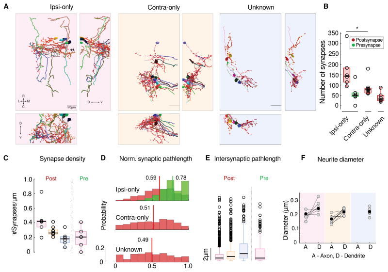
Figure 3
Integrator neuron projection patterns and synaptic distribution
(A) Colored panels show three views of reconstructed integrator neurons, grouped according to their axonal projection patterns. Left, 6 integrator neuron with ipsilateral projecting axons - ipsi-only ...

Figure 4
Integrator neurons organization and connectivity
(A) Planar organization of ipsi (pink) and contra (orange) projecting neurons postsynaptic sites. Grid represents the best fit plane through the cloud of points for each group. Anatomical landmarks, M...
Figure images are served from the NIH/NLM PubMed Central Open Access Subset or Europe PMC; copyright remains with the publishers and authors.
💬 Discussion
0 commentsNo comments yet. Be the first to start a discussion!
Leave a Comment