Abstract
Multiphoton microscopy has recently passed the milestone of its first 30 years of activity in biomedical research. The growing interest around this approach has led to a variety of applications from basic research to clinical practice. Moreover, this technique offers the advantage of label-free multiphoton imaging to analyze samples without staining processes and the need for a dedicated system. Here, we review the state of the art of label-free techniques; then, we focus on two-photon autofluorescence as well as second and third harmonic generation, describing physical and technical characteristics. We summarize some successful applications to a plethora of biomedical research fields and samples, underlying the versatility of this technique. A paragraph is dedicated to an overview of sample preparation, which is a crucial step in every microscopy experiment. Afterwards, we provide a detailed review analysis of the main quantitative methods to extract important information and parameters from acquired images using second harmonic generation. Lastly, we discuss advantages, limitations, and future perspectives in label-free multiphoton microscopy.
🔬 Techniques
✨ Fluorophores
🧪 Sample Preparation
💻 Software Details
🏛️ Research Organizations (ROR)
Affiliated research institutions:
📋 Methods
5.
Quantitative SHG Image Methods
Most published label-free multiphoton imaging studies took advantage of SHG to describe biological tissue organization from a qualitative point of view. Quantitative approaches were implemented only in the last few years. In the section below, we give a simplified summary of the analysis methods and the corresponding interpretation that can be associated with the multiphoton images (see Figure 3 and Figure 4 ). The methods are classified according to the features of the fibers that are possible to study: amount, texture, orientation, waviness, thickness, and distance. Some image properties (i.e., texture description and fibers orientation) can be treated with different approaches to extract similar and complementary information. The microscopic analysis can be run with ImageJ (with the Fiji image processing package, https://imagej.net/Fiji ) using different commercial or user-made plug-ins automatized with MATLAB and LabVIEW [ 18 , 52 , 71 , 72 ]. Table 2 summarizes the features and the approaches employed for image analysis and the corresponding degree of difficulty for each method according to the sophistication of the two-photon microscope and data analysis complexity. Table 2 assigns a higher degree of complexity to the set-up employed for the forward–backward SHG signal approach and the polarization method. Indeed, in both cases, a more sophisticated two-photon microscope is needed by introducing components and different detection pathways (see Section 5.2 ). The wavelet transformation method is more complex, since it is still a novelty for texture analysis and not very well implemented in commonly available software. 5.1. Amount and Texture Description 5.1.1. Intensity-Based Analysis → First-Order Statistics (FOS) In the first-order statistics, the intensities of individual pixels are considered independently from their neighboring pixels. Every pixel receives a value that is proportional to the detected signal, which can be associated with the amount of the fibers. Five first-order parameters (mean, standard deviation, integrated density, skewness, and kurtosis) are useful for SHG imaging analysis [ 18 , 52 , 71 ] (see Figure 3 a); the corresponding mathematical expression is described by Mustaço-Guidolin et al. and Haralick et al. [ 52 , 73 ]. The meaning and interpretation of the parameters are reported in Table 3 . According to Mostaço-Guidolin et al. [ 71 ], higher values of mean, integrated density, and standard deviation are associated with straight and thick fibers. Differently, curly and thin fibers are represented with higher kurtosis and skewness parameters. Any intermediate situation can be shown by median values of the five FOS parameters (see Figure 3 a). It is crucial to mention that FOS analysis is very sensitive to laser power variations, and comparison between different samples can be difficult. Monitoring laser power during the experiments is mandatory. → Second-Order Statistics (Gray Level Co-Occurrence Matrix, GLCM) The second-order statistics are based on inter-pixel correlation depending on the spatial arrangements of pixel intensities inside the region of interest. It is a measure of the probability of a pair of pixel values occurring at selected distances apart in the image, providing textural information for that region. This probability function is known as a co-occurrence matrix. Indeed, the most robust and frequently cited method for texture analysis is based on extracting various textural features from a gray level co-occurrence matrix (GLCM) [ 52 ]. The specific parameters most used are inverse difference moment (IDM), energy, inertia, entropy, and correlation, as reported in Table 4 . In Image-J, a specific plug-in called “GLCM texture” permits such analysis, and the corresponding mathematical expressions are described by Mustaço-Guidolin et al. and Haralick et al. [ 52 , 73 ]. In Figure 3 b, the radar plot shows the dependency of the GLCM parameters from the characteristics of the fibers. Correlation and IDM parameters do not show any significant trend according to the specific features of the tissue analyzed. Indeed, it is difficult to link some variations in the GLCM parameters directly to certain visual differences between the images [ 71 ]. In summary, first-order statistics (FOS) are parameters extracted directly from the original image while GLCM statistics are derived from a matrix that is built upon the inter-pixel correlation of the original image. Overall, Mostaço-Guidolin et al. demonstrated that the use of the full set of calculated texture parameters (combined FOS and GLCM) gives the best classification accuracy, at least in skin disorders [ 71 ]. 5.1.2. Transform-Based Methods → 2D Fast Fourier Transformation (2D-FFT) The transform-based texture analysis techniques convert the image into a new form using the spatial frequency properties of the pixel intensity variations allowing extracting textural characteristics from the image. Indhal and Næs [ 74 ] illustrated the use of two-dimensional Fast Fourier Transformation (2D-FFT) images for textural feature studies that can distinguish collagen fiber bundles with the same alignment. FFT has been by far the most used method to characterize SHG images due to its simplicity and availability in several image analysis software packages (see Figure 4 b). FFT analysis can be useful when combined with forward–backward SHG signal or polarization-resolved SHG images, as it provides a quantitative measure of fiber orientation (see Table 2 ) [ 75 , 76 , 77 ]. → Wavelet Transformation Wavelet transforms have been preferred recently in image texture analysis due to their space-frequency decomposition abilities. This method has been used to characterize and treat the problems of texture segmentation and classification [ 78 , 79 , 80 , 81 ]. Wavelet texture analysis methods currently appear to be the most powerful approach to image texture examination [ 82 ]. Indeed, two-dimensional wavelet transforms perform a space-frequency decomposition, which is more suitable than the frequency decomposition provided by the 2D FFT. The wavelet transform decomposes an image into four sub-images: low–low (LL), low–high (LH), high–low (HL), and high–high (HH). LL is the low-frequency sub-image that contains the main information of the decomposed image. LH, HL, and HH are three high-frequency sub-images that are horizontal, vertical, and oblique, respectively (see Figure 4 d). For an image with a coarse texture, the energy (from wavelet transformation) is mainly concentrated in the low-frequency sub-image, while for an image with a thin or complex texture, the energy is mainly concentrated in the high-frequency sub-image [ 82 ]. Nevertheless, it is complex to use due to the lack of a suitable and user-friendly implementation in common software. Further exploration of the capability of wavelets to help in the interpretation of SHG images is still needed. 5.2. Fibers Orientation → Forward–Backward SHG-Signal (F-SHG/B-SHG) F-SHG/B-SHG ratio measurements can be useful for assessing the fiber orientation content [ 77 , 83 ]. Laterally oriented fibers appear primarily in the backward direction, whereas axially oriented fibers appear primarily in the forward direction [ 18 ]. To successfully extract information from this measure, the relative collection efficiencies of the two detection pathways (forward and backward), including the detectors, need to be calibrated for each objective/condenser combination [ 18 , 41 ]. Typically, previous studies comparing both signals have relied on quantifying the ratio of their intensities (F-SHG/B-SHG ratio) [ 37 , 84 ]. For example, the F-SHG/B-SHG ratio has been used to assess the thickness of fibril shells and the ionic strength of the surrounding medium [ 84 ]. In other studies, the dependence of the F-SHG/B-SHG ratio on both the scattering properties of the tissue and the focal depth within the sample has been reported [ 37 ]. Probably, F-SHG/B-SHG ratio measurements are one of the most common quantitative measures presented in SHG image analysis. However, more rigorous experiments with standardized samples must be performed. → Polarization Polarization-resolved SHG is an alternative that can be used to extract information about the orientation of fibers in a certain image region; some authors presented examples of this type of SHG measurement [ 85 , 86 , 87 , 88 ]. The experiment can be in the form of measuring the intensity as a function of laser polarization or analyzing the signal anisotropy for constant linear polarization excitation [ 18 , 41 ]. In the first approach, at the beginning, the laser polarization is aligned with the long axis of collagen fiber(s), and then, images are typically acquired at least every 10° of laser polarization, through 180° of rotation. The intensities of the images are recorded at the starting point and after the rotation. This can be implemented by two methods, which are, in principle, physically equivalent. In the first, the specimen is fixed, and the polarization is rotated in the beam path with a λ/2 plate, or the second and more precise method is to place a polarization beamsplitting cube in the infinity space to select one linear polarization and then rotate the specimen for this excitation [ 41 ]. The second measurement determines the SH anisotropy by determination of SHG intensity detected after a laser polarizer oriented parallel and perpendicular to the laser polarization, respectively. Here, the linear polarization of the laser is fixed at 45° relative to the predominant fiber axis, and then in successive images, the SHG parallel and perpendicular components are measured relative to this excitation polarization [ 41 ]. At the molecular level, the polarization-sensitive second harmonic generation (PSHG) microscopy technique has been exploited by Psilodimitrakopoulos and colleagues [ 19 ] to uncover biological information non-accessible by intensity SHG analysis. In particular, using a pixel-level resolution analysis, they could retrieve polarization data on two different SHG active molecules (collagen and myosin) from the same image [ 20 ] or the helical pitch angle of amylopectin in starch [ 89 ]. → Coherency (C) The coherency parameter (C) permits estimating the local orientation of the fibers. The mathematical description for calculating C using OrientationJ, which is an ImageJ plug-in [ 72 ], is described by Rezakhaniha et al. [ 90 ]. Coherency is bounded between 0 and 1, with 1 indicating highly oriented structures and 0 indicating isotropic areas (see Figure 4 a). Recently, our group and collaborators calculated the coherency parameters for collagen and elastin to verify the local dominant orientation in representative regions of interest for bovine and porcine pericardia before and after the decellularization process [ 39 ]. 5.3. Fibers Waviness To quantify the waviness of fibers, a straightness parameter Ps is used, which is defined as the ratio of the distance between two points of the collagen bundle and the corresponding length [ 90 ]. Ps is bounded between 0 and 1; a bundle with Ps = 1 indicates a straight fiber; in contrast, Ps converges to zero when the fibers get very wavy ( Figure 4 c). The quantification of the fiber waviness can be done by using the ImageJ plugin NeuronJ, as reported in our previous studies [ 39 ]. 5.4. Fiber Thickness and Distance Such analysis can be done by selecting a region in the image or by simply drawing a line. Subsequently, by creating a plot profile, it is possible to extract distances between the peaks that can be associated with the distance between the fibers, and similarly, the widths of the peaks may give the thickness of them ( Figure 4 f).
Show full methods section
5.
Quantitative SHG Image Methods
Most published label-free multiphoton imaging studies took advantage of SHG to describe biological tissue organization from a qualitative point of view. Quantitative approaches were implemented only in the last few years. In the section below, we give a simplified summary of the analysis methods and the corresponding interpretation that can be associated with the multiphoton images (see Figure 3 and Figure 4 ). The methods are classified according to the features of the fibers that are possible to study: amount, texture, orientation, waviness, thickness, and distance. Some image properties (i.e., texture description and fibers orientation) can be treated with different approaches to extract similar and complementary information. The microscopic analysis can be run with ImageJ (with the Fiji image processing package, https://imagej.net/Fiji ) using different commercial or user-made plug-ins automatized with MATLAB and LabVIEW [ 18 , 52 , 71 , 72 ]. Table 2 summarizes the features and the approaches employed for image analysis and the corresponding degree of difficulty for each method according to the sophistication of the two-photon microscope and data analysis complexity. Table 2 assigns a higher degree of complexity to the set-up employed for the forward–backward SHG signal approach and the polarization method. Indeed, in both cases, a more sophisticated two-photon microscope is needed by introducing components and different detection pathways (see Section 5.2 ). The wavelet transformation method is more complex, since it is still a novelty for texture analysis and not very well implemented in commonly available software. 5.1. Amount and Texture Description 5.1.1. Intensity-Based Analysis → First-Order Statistics (FOS) In the first-order statistics, the intensities of individual pixels are considered independently from their neighboring pixels. Every pixel receives a value that is proportional to the detected signal, which can be associated with the amount of the fibers. Five first-order parameters (mean, standard deviation, integrated density, skewness, and kurtosis) are useful for SHG imaging analysis [ 18 , 52 , 71 ] (see Figure 3 a); the corresponding mathematical expression is described by Mustaço-Guidolin et al. and Haralick et al. [ 52 , 73 ]. The meaning and interpretation of the parameters are reported in Table 3 . According to Mostaço-Guidolin et al. [ 71 ], higher values of mean, integrated density, and standard deviation are associated with straight and thick fibers. Differently, curly and thin fibers are represented with higher kurtosis and skewness parameters. Any intermediate situation can be shown by median values of the five FOS parameters (see Figure 3 a). It is crucial to mention that FOS analysis is very sensitive to laser power variations, and comparison between different samples can be difficult. Monitoring laser power during the experiments is mandatory. → Second-Order Statistics (Gray Level Co-Occurrence Matrix, GLCM) The second-order statistics are based on inter-pixel correlation depending on the spatial arrangements of pixel intensities inside the region of interest. It is a measure of the probability of a pair of pixel values occurring at selected distances apart in the image, providing textural information for that region. This probability function is known as a co-occurrence matrix. Indeed, the most robust and frequently cited method for texture analysis is based on extracting various textural features from a gray level co-occurrence matrix (GLCM) [ 52 ]. The specific parameters most used are inverse difference moment (IDM), energy, inertia, entropy, and correlation, as reported in Table 4 . In Image-J, a specific plug-in called “GLCM texture” permits such analysis, and the corresponding mathematical expressions are described by Mustaço-Guidolin et al. and Haralick et al. [ 52 , 73 ]. In Figure 3 b, the radar plot shows the dependency of the GLCM parameters from the characteristics of the fibers. Correlation and IDM parameters do not show any significant trend according to the specific features of the tissue analyzed. Indeed, it is difficult to link some variations in the GLCM parameters directly to certain visual differences between the images [ 71 ]. In summary, first-order statistics (FOS) are parameters extracted directly from the original image while GLCM statistics are derived from a matrix that is built upon the inter-pixel correlation of the original image. Overall, Mostaço-Guidolin et al. demonstrated that the use of the full set of calculated texture parameters (combined FOS and GLCM) gives the best classification accuracy, at least in skin disorders [ 71 ]. 5.1.2. Transform-Based Methods → 2D Fast Fourier Transformation (2D-FFT) The transform-based texture analysis techniques convert the image into a new form using the spatial frequency properties of the pixel intensity variations allowing extracting textural characteristics from the image. Indhal and Næs [ 74 ] illustrated the use of two-dimensional Fast Fourier Transformation (2D-FFT) images for textural feature studies that can distinguish collagen fiber bundles with the same alignment. FFT has been by far the most used method to characterize SHG images due to its simplicity and availability in several image analysis software packages (see Figure 4 b). FFT analysis can be useful when combined with forward–backward SHG signal or polarization-resolved SHG images, as it provides a quantitative measure of fiber orientation (see Table 2 ) [ 75 , 76 , 77 ]. → Wavelet Transformation Wavelet transforms have been preferred recently in image texture analysis due to their space-frequency decomposition abilities. This method has been used to characterize and treat the problems of texture segmentation and classification [ 78 , 79 , 80 , 81 ]. Wavelet texture analysis methods currently appear to be the most powerful approach to image texture examination [ 82 ]. Indeed, two-dimensional wavelet transforms perform a space-frequency decomposition, which is more suitable than the frequency decomposition provided by the 2D FFT. The wavelet transform decomposes an image into four sub-images: low–low (LL), low–high (LH), high–low (HL), and high–high (HH). LL is the low-frequency sub-image that contains the main information of the decomposed image. LH, HL, and HH are three high-frequency sub-images that are horizontal, vertical, and oblique, respectively (see Figure 4 d). For an image with a coarse texture, the energy (from wavelet transformation) is mainly concentrated in the low-frequency sub-image, while for an image with a thin or complex texture, the energy is mainly concentrated in the high-frequency sub-image [ 82 ]. Nevertheless, it is complex to use due to the lack of a suitable and user-friendly implementation in common software. Further exploration of the capability of wavelets to help in the interpretation of SHG images is still needed. 5.2. Fibers Orientation → Forward–Backward SHG-Signal (F-SHG/B-SHG) F-SHG/B-SHG ratio measurements can be useful for assessing the fiber orientation content [ 77 , 83 ]. Laterally oriented fibers appear primarily in the backward direction, whereas axially oriented fibers appear primarily in the forward direction [ 18 ]. To successfully extract information from this measure, the relative collection efficiencies of the two detection pathways (forward and backward), including the detectors, need to be calibrated for each objective/condenser combination [ 18 , 41 ]. Typically, previous studies comparing both signals have relied on quantifying the ratio of their intensities (F-SHG/B-SHG ratio) [ 37 , 84 ]. For example, the F-SHG/B-SHG ratio has been used to assess the thickness of fibril shells and the ionic strength of the surrounding medium [ 84 ]. In other studies, the dependence of the F-SHG/B-SHG ratio on both the scattering properties of the tissue and the focal depth within the sample has been reported [ 37 ]. Probably, F-SHG/B-SHG ratio measurements are one of the most common quantitative measures presented in SHG image analysis. However, more rigorous experiments with standardized samples must be performed. → Polarization Polarization-resolved SHG is an alternative that can be used to extract information about the orientation of fibers in a certain image region; some authors presented examples of this type of SHG measurement [ 85 , 86 , 87 , 88 ]. The experiment can be in the form of measuring the intensity as a function of laser polarization or analyzing the signal anisotropy for constant linear polarization excitation [ 18 , 41 ]. In the first approach, at the beginning, the laser polarization is aligned with the long axis of collagen fiber(s), and then, images are typically acquired at least every 10° of laser polarization, through 180° of rotation. The intensities of the images are recorded at the starting point and after the rotation. This can be implemented by two methods, which are, in principle, physically equivalent. In the first, the specimen is fixed, and the polarization is rotated in the beam path with a λ/2 plate, or the second and more precise method is to place a polarization beamsplitting cube in the infinity space to select one linear polarization and then rotate the specimen for this excitation [ 41 ]. The second measurement determines the SH anisotropy by determination of SHG intensity detected after a laser polarizer oriented parallel and perpendicular to the laser polarization, respectively. Here, the linear polarization of the laser is fixed at 45° relative to the predominant fiber axis, and then in successive images, the SHG parallel and perpendicular components are measured relative to this excitation polarization [ 41 ]. At the molecular level, the polarization-sensitive second harmonic generation (PSHG) microscopy technique has been exploited by Psilodimitrakopoulos and colleagues [ 19 ] to uncover biological information non-accessible by intensity SHG analysis. In particular, using a pixel-level resolution analysis, they could retrieve polarization data on two different SHG active molecules (collagen and myosin) from the same image [ 20 ] or the helical pitch angle of amylopectin in starch [ 89 ]. → Coherency (C) The coherency parameter (C) permits estimating the local orientation of the fibers. The mathematical description for calculating C using OrientationJ, which is an ImageJ plug-in [ 72 ], is described by Rezakhaniha et al. [ 90 ]. Coherency is bounded between 0 and 1, with 1 indicating highly oriented structures and 0 indicating isotropic areas (see Figure 4 a). Recently, our group and collaborators calculated the coherency parameters for collagen and elastin to verify the local dominant orientation in representative regions of interest for bovine and porcine pericardia before and after the decellularization process [ 39 ]. 5.3. Fibers Waviness To quantify the waviness of fibers, a straightness parameter Ps is used, which is defined as the ratio of the distance between two points of the collagen bundle and the corresponding length [ 90 ]. Ps is bounded between 0 and 1; a bundle with Ps = 1 indicates a straight fiber; in contrast, Ps converges to zero when the fibers get very wavy ( Figure 4 c). The quantification of the fiber waviness can be done by using the ImageJ plugin NeuronJ, as reported in our previous studies [ 39 ]. 5.4. Fiber Thickness and Distance Such analysis can be done by selecting a region in the image or by simply drawing a line. Subsequently, by creating a plot profile, it is possible to extract distances between the peaks that can be associated with the distance between the fibers, and similarly, the widths of the peaks may give the thickness of them ( Figure 4 f).
5.1.2. Transform-Based Methods → 2D Fast Fourier Transformation (2D-FFT) The transform-based texture analysis techniques convert the image into a new form using the spatial frequency properties of the pixel intensity variations allowing extracting textural characteristics from the image. Indhal and Næs [ 74 ] illustrated the use of two-dimensional Fast Fourier Transformation (2D-FFT) images for textural feature studies that can distinguish collagen fiber bundles with the same alignment. FFT has been by far the most used method to characterize SHG images due to its simplicity and availability in several image analysis software packages (see Figure 4 b). FFT analysis can be useful when combined with forward–backward SHG signal or polarization-resolved SHG images, as it provides a quantitative measure of fiber orientation (see Table 2 ) [ 75 , 76 , 77 ]. → Wavelet Transformation Wavelet transforms have been preferred recently in image texture analysis due to their space-frequency decomposition abilities. This method has been used to characterize and treat the problems of texture segmentation and classification [ 78 , 79 , 80 , 81 ]. Wavelet texture analysis methods currently appear to be the most powerful approach to image texture examination [ 82 ]. Indeed, two-dimensional wavelet transforms perform a space-frequency decomposition, which is more suitable than the frequency decomposition provided by the 2D FFT. The wavelet transform decomposes an image into four sub-images: low–low (LL), low–high (LH), high–low (HL), and high–high (HH). LL is the low-frequency sub-image that contains the main information of the decomposed image. LH, HL, and HH are three high-frequency sub-images that are horizontal, vertical, and oblique, respectively (see Figure 4 d). For an image with a coarse texture, the energy (from wavelet transformation) is mainly concentrated in the low-frequency sub-image, while for an image with a thin or complex texture, the energy is mainly concentrated in the high-frequency sub-image [ 82 ]. Nevertheless, it is complex to use due to the lack of a suitable and user-friendly implementation in common software. Further exploration of the capability of wavelets to help in the interpretation of SHG images is still needed.
📊 Figures
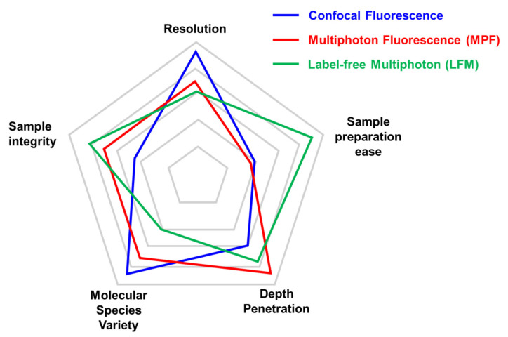
Figure 1
Comparison of key parameters of different imaging techniques. Each microscopy technique has strengths and weaknesses that are important to consider before choosing the adequate microscopy approach. We...
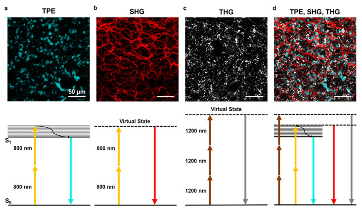
Figure 2
Two-photon excitation, second and third harmonic generation. ( a ) Example of two-photon excitation (TPE) of DAPI stained nuclei in lung tissue. Bottom panel shows the corresponding Jablonski diagram ...
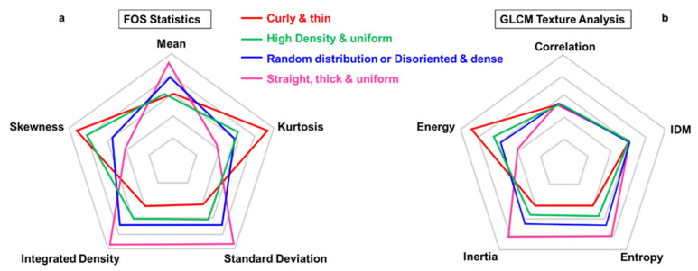
Figure 3
Radar plots for first-order statistics (FOS) and second-order statistics (gray level co-occurrence matrix, GLCM). Comparison of the statistical parameters between four categories of typical fibers arr...
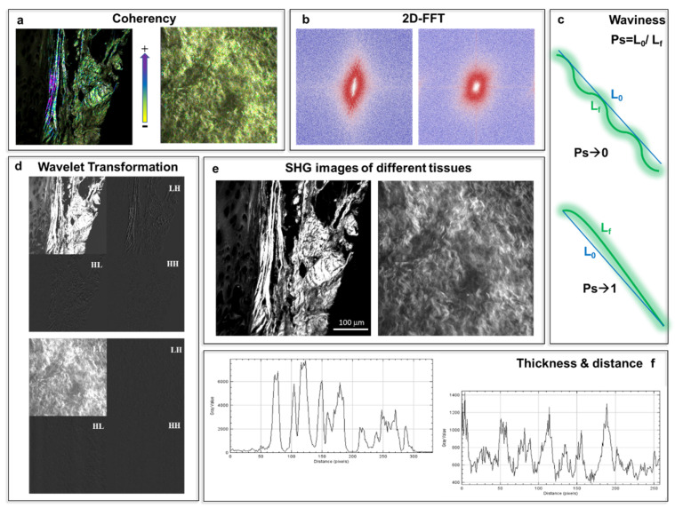
Figure 4
Analysis of SHG images of native and decellularized tissue ( e ) using ImageJ software. ( a ) Coherency analysis showing different values between 0 and 1 with 1 indicating a highly orientated structur...
Figure images are served from the NIH/NLM PubMed Central Open Access Subset or Europe PMC; copyright remains with the publishers and authors.
💬 Discussion
0 commentsNo comments yet. Be the first to start a discussion!
Leave a Comment