Abstract
Counting cells and colonies is an integral part of high-throughput screens and quantitative cellular assays. Due to its subjective and time-intensive nature, manual counting has hindered the adoption of cellular assays such as tumor spheroid formation in high-throughput screens. The objective of this study was to develop an automated method for quick and reliable counting of cells and colonies from digital images. For this purpose, I developed an ImageJ macro Cell Colony Edge and a CellProfiler Pipeline Cell Colony Counting, and compared them to other open-source digital methods and manual counts. The ImageJ macro Cell Colony Edge is valuable in counting cells and colonies, and measuring their area, volume, morphology, and intensity. In this study, I demonstrate that Cell Colony Edge is superior to other open-source methods, in speed, accuracy and applicability to diverse cellular assays. It can fulfill the need to automate colony/cell counting in high-throughput screens, colony forming assays, and cellular assays.
🔬 Techniques
🧬 Organisms
💻 Software
✨ Fluorophores
🧪 Sample Preparation
🔬 Cell Lines
🏭 Microscope Brands
🧪 Reagent Suppliers
💻 Software Details
🏛️ Research Organizations (ROR)
Affiliated research institutions:
📋 Methods
Cell Culture
All experiments were performed under standard cell culture conditions at 37°C and 5% CO 2 . The human breast cancer line T47D was purchased from the American Type Culture Collection (Manassas, VA). Cells were cultured in RPMI 1640 medium (Sigma-Aldrich, St Louis) supplemented with 10% fetal bovine serum (Invitrogen, Carlsbad) and 1% penicillin-streptomycin (Gibco-Invitrogen Inc). For tumorsphere assays, 25,000 cells were grown in 3% methylcellulose (Sigma-Aldrich) in triplicate in 6-well dishes coated with Poly (2-hydroxyethyl methacrylate) (Sigma-Aldrich). Imaging was done after two weeks of culture. For clonogenic assays, 10 5 T47D cells were grown overnight and exposed to 0–8 Gy irradiation. A total of 1,000 cells were seeded in triplicate into 6-well tissue culture plates.
Bacterial cell plating
Escherichia coli were grown on 100mm LB plates at various dilutions overnight at 37°C. IMJ Cell Colony Edge The general IMJ Edge macro with prompts for user input is given in S1 Appendix . It is also available for download from https://sourceforge.net/projects/cell-colony-edge/files/ . The parameters used for different analyses are also given. It is quite long, but the user can customize and simplify it for their purposes. Customized versions of IMJ Edge for different images and resolutions (for example, bacterial versus clonogenic assay), and are given in S2 Appendix . The tunable values such as minimum and maximum size were based on manual measurements, and are shown in red. S1 Fig shows an example of how tunable parameters are determined by trial and error for an image of a single cell (courtesy [ 40 ]). S3 Appendix gives the steps for manual trial and error using the ImageJ GUI. S4 Appendix gives instructions for downloading and using the macro. The macro has six major steps: 1) Background subtraction, 2) Sharpening and Finding Edges, 3) Smoothing and converting to black and white, 4) Closing and filling holes, 5) Denoising and segmenting, 6) Filtering and Measuring ( Fig 1 ). 1) First, the background is subtracted to enhance contrast and reduce effects of uneven illumination (Figure B in S1 Fig ). The radius for Background subtraction was determined empirically. A starting number can be the average radius of colonies. 2) Since the macro relies on edge detection, the next step is sharpening and enhancing the image, followed by finding the edges (Figure C in S1 Fig ). ImageJ’s in-built Sobel filter is used in the macro. Users are welcome to download and use Canny edge detection or LoG filter. 3) The image is smoothened (Gaussian Blur), and converted to black and white (Make Binary) (Figure D in S1 Fig ). Alternatively, the image can be smoothened by sequential dilate and erode steps. 4) This is followed by closing of the edges to form closed circle/ellipses (Close), closed objects are filled black (Fill Holes), resulting in images containing black colonies on a white background (Figure D in S1 Fig ). To ensure that all colonies are detected, an additional step of closing and filling holes is performed. Here, the size of each pixel is increased (Maximum) (Figure E in S1 Fig ), in order to bring the detected edges closer to each other, followed by closing and filling (Figure F in S1 Fig ). This step allows the detection of colonies whose entire edge along the perimeter fails to be otherwise detected. After filling, the size of the pixels is reduced (Minimum), returning the colony size to their original values (Figure G in S1 Fig ). The pixel sizes for this step have to be chosen manually based on the resolution of the images and the size of the colonies. Note that these expanding and shrinking steps were not required for measurement of bacterial colonies. 5) The final steps involve denoising and segmentation, to remove small particles (artifacts) and to separate clustered colonies. S1 Fig focuses on a single cell for clarity, and hence denoising and segmentation steps are not shown. Denoising is done by deselection of particles (Remove Outliers) smaller than a manually set threshold. This step can be performed multiple times with different thresholds. For example, due to small size of bacterial colonies, artefacts such as scratch marks on the plate become very prominent during the closing and filling holes steps. Hence a couple of Remove Outliers steps were inserted before the smoothing step to exclude these false positives ( S2 Appendix ). 6) Finally, the objects are filtered based on size, circularity, closeness to edge etc, and only objects meeting the user defined criteria are measured. For intensity measurements, such as in clonogenic assays, the ROI’s (Regions Of Interest) can be redirected to the original image, via the ROI manager, and then measured ( S1 Appendix ). CellProfiler Pipeline: Cell Colony Counting A new pipeline was made for detection of cells and colonies from brightfield/nomarski images ( https://sourceforge.net/projects/cell-colony-edge/files/ ). This pipeline has four major steps: 1) Background correction, 2) Colony detection & Filtering, 3) Measuring Colony parameters, 4) Overlaying and saving images ( Fig 1 ). Background correction is done through its own inherent modules- Color to Gray, Correct Illumination calculation, and Correct Illumination Apply. Modules for object detection (Identify Primary Objects) based on thresholding are available in Cell Profiler. While ImageJ allows filtering at the measuring stage, the primary objects have to be filtered first in Cell Profiler. Hence, the subsequent steps involved measuring the size and shape of the object, followed by filtration based on form factor and size. After filtering, the object’s size, shape and intensity are measured again, outlines of filtered objects are overlaid on the original image and saved.
Show full methods section
Cell Culture
All experiments were performed under standard cell culture conditions at 37°C and 5% CO 2 . The human breast cancer line T47D was purchased from the American Type Culture Collection (Manassas, VA). Cells were cultured in RPMI 1640 medium (Sigma-Aldrich, St Louis) supplemented with 10% fetal bovine serum (Invitrogen, Carlsbad) and 1% penicillin-streptomycin (Gibco-Invitrogen Inc). For tumorsphere assays, 25,000 cells were grown in 3% methylcellulose (Sigma-Aldrich) in triplicate in 6-well dishes coated with Poly (2-hydroxyethyl methacrylate) (Sigma-Aldrich). Imaging was done after two weeks of culture. For clonogenic assays, 10 5 T47D cells were grown overnight and exposed to 0–8 Gy irradiation. A total of 1,000 cells were seeded in triplicate into 6-well tissue culture plates.
Bacterial cell plating
Escherichia coli were grown on 100mm LB plates at various dilutions overnight at 37°C. IMJ Cell Colony Edge The general IMJ Edge macro with prompts for user input is given in S1 Appendix . It is also available for download from https://sourceforge.net/projects/cell-colony-edge/files/ . The parameters used for different analyses are also given. It is quite long, but the user can customize and simplify it for their purposes. Customized versions of IMJ Edge for different images and resolutions (for example, bacterial versus clonogenic assay), and are given in S2 Appendix . The tunable values such as minimum and maximum size were based on manual measurements, and are shown in red. S1 Fig shows an example of how tunable parameters are determined by trial and error for an image of a single cell (courtesy [ 40 ]). S3 Appendix gives the steps for manual trial and error using the ImageJ GUI. S4 Appendix gives instructions for downloading and using the macro. The macro has six major steps: 1) Background subtraction, 2) Sharpening and Finding Edges, 3) Smoothing and converting to black and white, 4) Closing and filling holes, 5) Denoising and segmenting, 6) Filtering and Measuring ( Fig 1 ). 1) First, the background is subtracted to enhance contrast and reduce effects of uneven illumination (Figure B in S1 Fig ). The radius for Background subtraction was determined empirically. A starting number can be the average radius of colonies. 2) Since the macro relies on edge detection, the next step is sharpening and enhancing the image, followed by finding the edges (Figure C in S1 Fig ). ImageJ’s in-built Sobel filter is used in the macro. Users are welcome to download and use Canny edge detection or LoG filter. 3) The image is smoothened (Gaussian Blur), and converted to black and white (Make Binary) (Figure D in S1 Fig ). Alternatively, the image can be smoothened by sequential dilate and erode steps. 4) This is followed by closing of the edges to form closed circle/ellipses (Close), closed objects are filled black (Fill Holes), resulting in images containing black colonies on a white background (Figure D in S1 Fig ). To ensure that all colonies are detected, an additional step of closing and filling holes is performed. Here, the size of each pixel is increased (Maximum) (Figure E in S1 Fig ), in order to bring the detected edges closer to each other, followed by closing and filling (Figure F in S1 Fig ). This step allows the detection of colonies whose entire edge along the perimeter fails to be otherwise detected. After filling, the size of the pixels is reduced (Minimum), returning the colony size to their original values (Figure G in S1 Fig ). The pixel sizes for this step have to be chosen manually based on the resolution of the images and the size of the colonies. Note that these expanding and shrinking steps were not required for measurement of bacterial colonies. 5) The final steps involve denoising and segmentation, to remove small particles (artifacts) and to separate clustered colonies. S1 Fig focuses on a single cell for clarity, and hence denoising and segmentation steps are not shown. Denoising is done by deselection of particles (Remove Outliers) smaller than a manually set threshold. This step can be performed multiple times with different thresholds. For example, due to small size of bacterial colonies, artefacts such as scratch marks on the plate become very prominent during the closing and filling holes steps. Hence a couple of Remove Outliers steps were inserted before the smoothing step to exclude these false positives ( S2 Appendix ). 6) Finally, the objects are filtered based on size, circularity, closeness to edge etc, and only objects meeting the user defined criteria are measured. For intensity measurements, such as in clonogenic assays, the ROI’s (Regions Of Interest) can be redirected to the original image, via the ROI manager, and then measured ( S1 Appendix ). CellProfiler Pipeline: Cell Colony Counting A new pipeline was made for detection of cells and colonies from brightfield/nomarski images ( https://sourceforge.net/projects/cell-colony-edge/files/ ). This pipeline has four major steps: 1) Background correction, 2) Colony detection & Filtering, 3) Measuring Colony parameters, 4) Overlaying and saving images ( Fig 1 ). Background correction is done through its own inherent modules- Color to Gray, Correct Illumination calculation, and Correct Illumination Apply. Modules for object detection (Identify Primary Objects) based on thresholding are available in Cell Profiler. While ImageJ allows filtering at the measuring stage, the primary objects have to be filtered first in Cell Profiler. Hence, the subsequent steps involved measuring the size and shape of the object, followed by filtration based on form factor and size. After filtering, the object’s size, shape and intensity are measured again, outlines of filtered objects are overlaid on the original image and saved.
Image Acquisition and Analysis
Images of tumorspheres were acquired using brightfield microscopy with a 5X objective (Nikon C1si, Nikon Instruments Inc., Melville, NY, USA). Bacterial plates and 6-well plates in clonogenic assays were imaged using a digital camera that could capture the entire plate area in a single image. Images were were cropped and saved as a folder of.tiff files. For clonogenic assays, the area outside the plate was set to background color. The scale of images was determined using a calibration slide. Images were analyzed using the open-source softwares ImageJ (Fiji package)–IMJ Cai and IMJ Edge macro, OpenCFU and CellProfiler. For manual measurements of colony area and perimeter, ImageJ’s ‘draw ellipse’ and ‘measure’ (Analyze-Measure) tools were used for each colony on the original image. The optimal parameters were determined for each method by trial and error, and measurements of detected objects recorded. The parameters for IMJ Cai were optimized manually as per directions provided in Cai et al [ 28 ]. For each method (including manual), images were analyzed five times, and the average values used. To compare the accuracy of various methods, the measurements of the detected objects from various methods were compared to manual measurements. Detected objects from various methods were matched manually by either printing the labeled processed images, using the x-y coordinates and area measurements, or selecting colonies in the software. If an automated method segmented a colony into parts, then the largest segment was matched with the manual measurement of the full colony. The smaller colony was given an additional colony number. If an automated method did not segment two touching colonies, then that merged colony was matched to the larger of the two manually segmented colonies. The smaller of the two manually segmented colonies was counted as an additional colony, undetected by that automated method. Results from area and perimeter measurement were analyzed in MS Excel. Boxplots were made in R.
Supporting Information S1 Appendix ImageJ Cell_Colony_Edge Macro. The macro given in text. The text in green explains the function of the following code. The parameters used for different images are also given. (PDF) Click here for additional data file. S2 Appendix Customized versions of Cell_Colony_Edge macro for specific purposes. (PDF) Click here for additional data file. S3 Appendix Instructions for manual determination of parameters using ImageJ GUI. (PDF) Click here for additional data file. S4 Appendix Instructions for downloading and running the macro. (PDF) Click here for additional data file. S1 Fig Image Processing steps of IMJ Edge, and selection of parameters. (Figure A) Original Nomarksi image showing a single U266 cell (modified from [ 40 ]). The diameter was measured as 10 px in ImageJ. (Figure B) Image in (A) after background subtraction with different rolling ball radii (written in bottom right corner of each image). Rolling ball radius of 40 was selected (blue checkmark) because all edges were visible. (Figure C) Background subtracted image is then sharpened and enhanced (0.2%). This image is further processed by the “Find Edges” and “Make Binary” commands. (Figure D) The binary image is processed by the “Gaussian blur” command with different sigma radii (written in bottom right corner of each image), followed by filling and closing of holes. Red arrows show that debris is processed as an object when 0.25 or 1 is used as radius for Gaussian blur. Gaussian blur with radius 2 did not select debris as an object, and was selected (blue checkmark). (Figure E) Closed and Filled image in D is further processed by the “Maximum” command to increase size of each pixel. This brings the edges of gaps closer together (green arrows). Radius 2 was selected, as the edges of gap are close enough for filling and closing. (Figure F) Image in E was closed and filled. (Figure G) Size of pixels is reduced back. Radius 5 is chosen because size of selection is similar to the size of cell in original image. Overlay is shown for comparison purposes. (TIFF) Click here for additional data file. S2 Fig Variability in Manual measurement of bacterial colonies. The plot is broken in two halves with different scales to represent different values on the y-axes with Colony numbers on the x-axis. (TIF) Click here for additional data file. S3 Fig Other methods of colony counting not tested in paper. (Figure A) Original image of tumorspheres processed by different methods. (Figure B) Results of image processed by Sieuwerts et al ImageJ plugin. Vertical arrows point to undetected colonies, and horizontal to colonies that are only partly detected. (Figure C) Image of Clonocounter working on Image in Figure A. Only part of the image inside the circle is analyzed. In this part too, the green highlights show the detected colonies. The table underneath shows the results of clonocounter. (Figure D) Original tumorsphere image on the left followed by the image processed by Treloar and Simpson ImageJ method and by IMJEdge. (TIF) Click here for additional data file.
📊 Figures
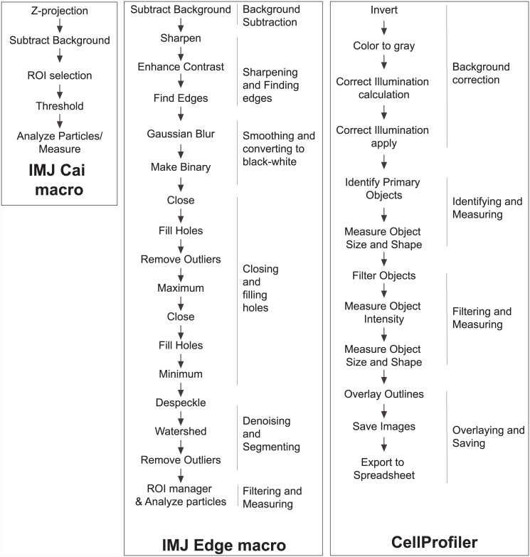
Fig 1
Flowchart representing the processing steps in different Colony detection methods.
OpenCFUu2019s flowchart is not shown here.
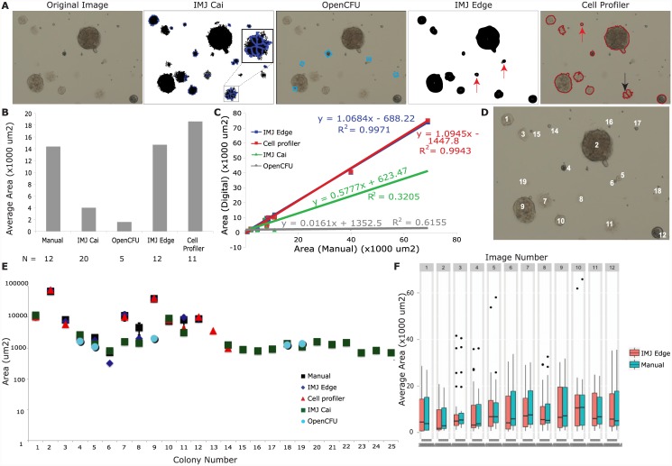
Fig 2
Comparison of different digital colony detection methods with manual measurements for tumorspheres.
The first image in (A) is the original image. The rest are processed images from the colony detection methods. IMJ Cai has the thresholded areas in black, while the detected colonies have a blue outli...
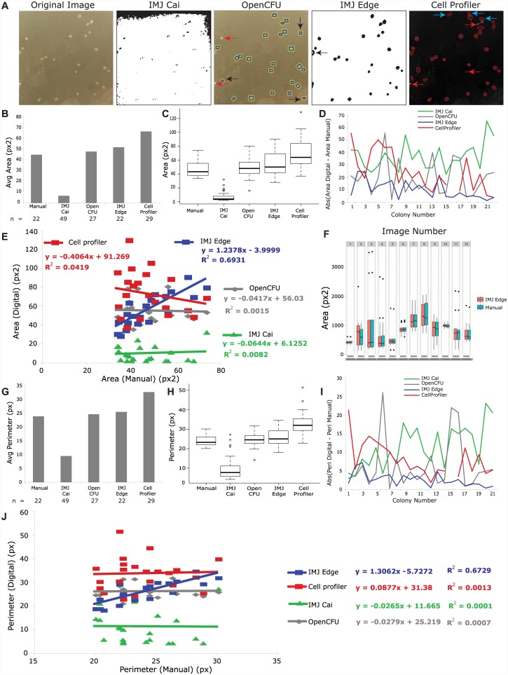
Fig 3
Comparison of digital methods for colony detection for bacterial colonies.
(A) shows the original image, and masks/overlays of detected colonies by various methods. (B) Plot of the average of area measurements, while (C) is boxplot showing the distribution of area measuremen...
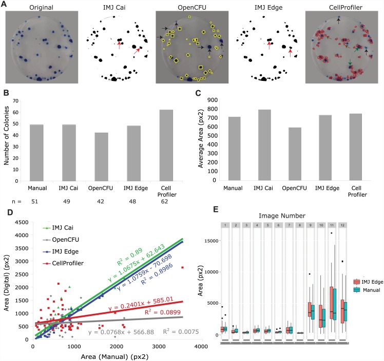
Fig 4
Comparison of digital methods for colony detection for bacterial colonies.
(A) shows the original image, and masks/overlays of detected colonies by various methods. Red arrows in IMJ Cai and IMJ Edge mark unsegmented colonies. Black arrows mark undetected colonies. (B) Plot ...
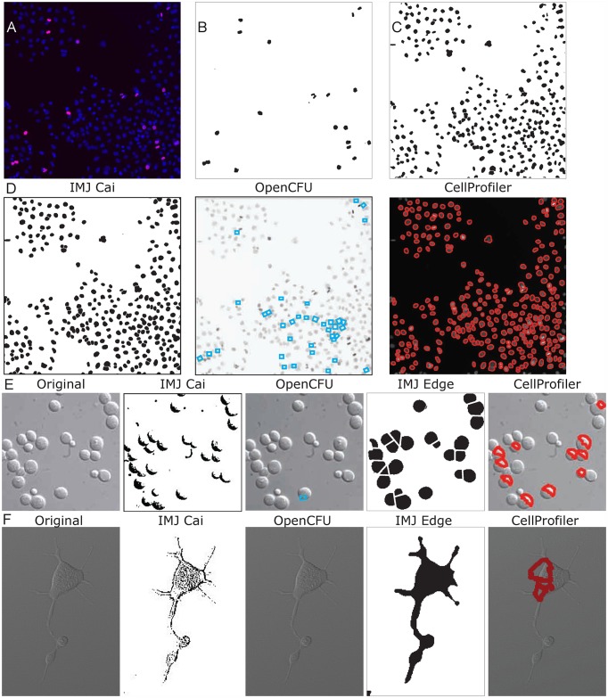
Fig 5
Application of IMJ Edge for detection of cells.
(A) RGB image showing DAPI staining of nuclei in blue, and phospho-histone3 staining in red. (B) shows the red channel processed with IMJ Edge to calculate the number of dividing cells. (C) shows the ...
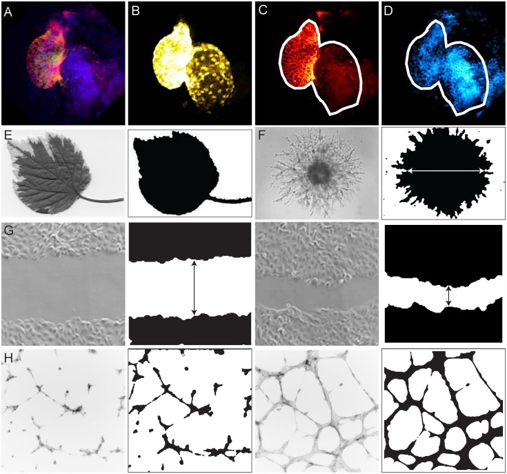
Fig 6
Application of IMJ Edge on tissue images and cellular assays.
(A) Image of a stained zebrafish heart with heart cells in green ( cmcl2 : gfp line), nuclei in blue (DAPI), and heart cell membranes stained in red (Alcama antibody). The green channel (B) was proces...
Figure images are served from the NIH/NLM PubMed Central Open Access Subset or Europe PMC; copyright remains with the publishers and authors.
💬 Discussion
0 commentsNo comments yet. Be the first to start a discussion!
Leave a Comment