Abstract
Calcium imaging with fluorescent protein sensors is widely used to record activity in neuronal populations. The transform between neural activity and calcium-related fluorescence involves nonlinearities and low-pass filtering, but the effects of the transformation on analyses of neural populations are not well understood. We compared neuronal spikes and fluorescence in matched neural populations in behaving mice. We report multiple discrepancies between analyses performed on the two types of data, including changes in single-neuron selectivity and population decoding. These were only partially resolved by spike inference algorithms applied to fluorescence. To model the relation between spiking and fluorescence we simultaneously recorded spikes and fluorescence from individual neurons. Using these recordings we developed a model transforming spike trains to synthetic-imaging data. The model recapitulated the differences in analyses. Our analysis highlights challenges in relating electrophysiology and imaging data, and suggests forward modeling as an effective way to understand differences between these data.
🔬 Techniques
🔭 Microscopes
✨ Fluorophores
🧪 Sample Preparation
🔬 Cell Lines
🏭 Microscope Brands
🧪 Reagent Suppliers
📋 Protocols
💻 Code & Software
Public API for neural recording methodology comparison, including all relevant modules
A list of existing calcium imaging deconvolution methods
This is a developing website for our project of neural recording methodologies comparison.
💾 Data Repositories
🏛️ Research Organizations (ROR)
Affiliated research institutions:
📋 Methods
Electrophysiological and imaging population activity recordings Electrophysiological (‘ephys’)[ 25 ] or calcium imaging[ 25 , 36 ] recordings were performed in separate experiments and described in detail in the original publications ( S1 Table ; http://im-phys.org/data ). Mice were trained to perform a delayed version of a tactile discrimination task. Mice reported the position of a pole (anterior or posterior) by directional licking (lick-left or lick-right) after a delay period. The duration of sample and delay epoch was 2.6 s. In ephys, the delay epoch was 1.3 s; in imaging, it was 1.4 s. Trials with early licking were excluded from analysis. Neuronal depths were 100 to 800 um (ephys), 150–740 um (6s-AAV), 120–640 um (Thy1-GP4.3 mice, 6s-TG), and 140–470 um (Thy1-GP5.17 mice, 6f-TG). Only sessions with more than 20 trials for each type (right-trial and left-trial) were included. For imaging data, we performed a post-hoc detection of outliers and removed trials where more than 30% of the time points contain a signal with 3 standard deviations away from median (these outliers relate to baseline fluctuations across trials, and removing them was necessary for variance-based analysis). Neurons were limited to putative pyramidal neurons. These reduced the total number of neurons with sufficient number of trials, yielding 1493, 2293, and 2672 units for 6s-AAV, 6s-TG and 6f-TG imaging, respectively. We note that despite the 6s-TG data containing many neurons across multiple sessions all data came from a single animal. Though we find this data to be consistent with other imaging data, the single animal source could be a potential issue in that differences in an individual animal’s behavior may cause differences in neural encoding. We used two sets of data from loose-seal electrophysiological recordings and imaging from GCaMP6-expressing neurons in primary visual cortex. In one set neurons were transduced with 6s-AAV and 6f-AAV (data from[ 13 ]). For 6s-AAV data, imaging was performed after 2–4 weeks of expression. In the other set we used 6s-TG and 6f-TG mice[ 31 , 69 ]. More details of all datasets are described at http://im-phys.org/data . In the imaging data, individual neurons were visually identified based on average fluorescence images as well as “neighborhood correlation maps” (where the brightness of each pixel encodes the correlation of its fluorescent time course to that of its neighbors), which highlights active cells. Each ROI was inspected to correspond to a morphological neuron and have a generally donut-like shape (since the nucleus does not express the indicator). The fluorescence time course of each cell was measured by averaging all pixels within the ROI, with a correction for neuropil contamination. The fluorescence signal of a cell body was estimated as F cell (t) = F roi (t)-r*F neuropil (t), with r = 0.7. The neuropil signal F neuropil (t) surrounding each cell was measured by averaging the signal of all pixels within a 40 μm radius from the cell center (excluding all selected cells). For each imaging plane, the number of ROIs was about 30+/-19 cells in the 6s-AAV imaging conditions, and 82+/-48 cells per recording plane in 6s-TG, and 122+/-32 cells per recording plane in 6f-TG. Whole-cell recordings were made using pulled borosilicate glass (Sutter instrument). A small craniotomy (100–300 μm diameter) was created over the ALM (bregma AP 0.0 mm, ML 2.0 mm) under isofluorane anaesthesia and covered with cortex buffer during recording. Whole-cell patch pipettes (7–9 MΩ) were filled with internal solution (in mM): 135 K-gluconate, 4 KCl, 10 HEPES, 0.5 EGTA, 10 Na 2 -phosphocreatine, 4 Mg-ATP, 0.4 Na2-GTP and 0.3% Biocytin (293–303 mOsm, pH 7.3). The membrane potential, V m , was amplified (Multiclamp 700B, Molecular Devices) and sampled at 20 kHz using WaveSurfer ( http://wavesurfer.janelia.org/ ). V m were not corrected for liquid junction potential. After the recording the craniotomy was covered with Kwik-Cast (World Precision Instruments). Each animal was used for 2–3 recording sessions. Recordings were made from 350 to 850 μm below the pia. Simultaneous loose-seal recordings and imaging ( Figs 3 and S2 ; S2 Table ) was performed as described previously[ 13 ] (more details at http://im-phys.org/data ). GP4.3 and GP5.17 mice[ 31 ] were lightly anesthetized (0.5% isoflurane). Drifting grating visual stimuli were used to drive activity in the visual cortex. Loose-seal recordings were made through a craniotomy windows over the primary visual cortex. Two-photon imaging and loose-seal, cell-attached recordings were performed simultaneously. We acquired images in both low (284 x 284 um 2 ) and high (38 x 38 um 2 ) zoom configurations. Extraction of fluorescence transients was as described[ 13 ]. All procedures in mice experiments were performed in compliance with the Janelia Research Campus Institutional Animal Care and Use Committee. To analyze the spike-triggered fluorescence changes, we created 1.2-s snippets around action potentials (APs), where a few APs only happened from 200 ms to 400 ms from the onset of each snippet. We computed baseline fluorescence using the snippets without AP in the entire time series. For snippet with APs, we required the fluorescence changes within the first 200 ms (before APs) was around baseline level ( Fig 3C and S2A ). We computed ROC curves for detecting one ( Fig 3E , inset panels) or many APs ( Figs 3E and S2C ) compared to baseline fluorescence fluctuations. D-prime was computed as < max ( Δ F / F ) 1 A P > − < max ( Δ F / F ) n o A P > std ( Δ F / F ) n o A P .
Show full methods section
Electrophysiological and imaging population activity recordings Electrophysiological (‘ephys’)[ 25 ] or calcium imaging[ 25 , 36 ] recordings were performed in separate experiments and described in detail in the original publications ( S1 Table ; http://im-phys.org/data ). Mice were trained to perform a delayed version of a tactile discrimination task. Mice reported the position of a pole (anterior or posterior) by directional licking (lick-left or lick-right) after a delay period. The duration of sample and delay epoch was 2.6 s. In ephys, the delay epoch was 1.3 s; in imaging, it was 1.4 s. Trials with early licking were excluded from analysis. Neuronal depths were 100 to 800 um (ephys), 150–740 um (6s-AAV), 120–640 um (Thy1-GP4.3 mice, 6s-TG), and 140–470 um (Thy1-GP5.17 mice, 6f-TG). Only sessions with more than 20 trials for each type (right-trial and left-trial) were included. For imaging data, we performed a post-hoc detection of outliers and removed trials where more than 30% of the time points contain a signal with 3 standard deviations away from median (these outliers relate to baseline fluctuations across trials, and removing them was necessary for variance-based analysis). Neurons were limited to putative pyramidal neurons. These reduced the total number of neurons with sufficient number of trials, yielding 1493, 2293, and 2672 units for 6s-AAV, 6s-TG and 6f-TG imaging, respectively. We note that despite the 6s-TG data containing many neurons across multiple sessions all data came from a single animal. Though we find this data to be consistent with other imaging data, the single animal source could be a potential issue in that differences in an individual animal’s behavior may cause differences in neural encoding. We used two sets of data from loose-seal electrophysiological recordings and imaging from GCaMP6-expressing neurons in primary visual cortex. In one set neurons were transduced with 6s-AAV and 6f-AAV (data from[ 13 ]). For 6s-AAV data, imaging was performed after 2–4 weeks of expression. In the other set we used 6s-TG and 6f-TG mice[ 31 , 69 ]. More details of all datasets are described at http://im-phys.org/data . In the imaging data, individual neurons were visually identified based on average fluorescence images as well as “neighborhood correlation maps” (where the brightness of each pixel encodes the correlation of its fluorescent time course to that of its neighbors), which highlights active cells. Each ROI was inspected to correspond to a morphological neuron and have a generally donut-like shape (since the nucleus does not express the indicator). The fluorescence time course of each cell was measured by averaging all pixels within the ROI, with a correction for neuropil contamination. The fluorescence signal of a cell body was estimated as F cell (t) = F roi (t)-r*F neuropil (t), with r = 0.7. The neuropil signal F neuropil (t) surrounding each cell was measured by averaging the signal of all pixels within a 40 μm radius from the cell center (excluding all selected cells). For each imaging plane, the number of ROIs was about 30+/-19 cells in the 6s-AAV imaging conditions, and 82+/-48 cells per recording plane in 6s-TG, and 122+/-32 cells per recording plane in 6f-TG. Whole-cell recordings were made using pulled borosilicate glass (Sutter instrument). A small craniotomy (100–300 μm diameter) was created over the ALM (bregma AP 0.0 mm, ML 2.0 mm) under isofluorane anaesthesia and covered with cortex buffer during recording. Whole-cell patch pipettes (7–9 MΩ) were filled with internal solution (in mM): 135 K-gluconate, 4 KCl, 10 HEPES, 0.5 EGTA, 10 Na 2 -phosphocreatine, 4 Mg-ATP, 0.4 Na2-GTP and 0.3% Biocytin (293–303 mOsm, pH 7.3). The membrane potential, V m , was amplified (Multiclamp 700B, Molecular Devices) and sampled at 20 kHz using WaveSurfer ( http://wavesurfer.janelia.org/ ). V m were not corrected for liquid junction potential. After the recording the craniotomy was covered with Kwik-Cast (World Precision Instruments). Each animal was used for 2–3 recording sessions. Recordings were made from 350 to 850 μm below the pia. Simultaneous loose-seal recordings and imaging ( Figs 3 and S2 ; S2 Table ) was performed as described previously[ 13 ] (more details at http://im-phys.org/data ). GP4.3 and GP5.17 mice[ 31 ] were lightly anesthetized (0.5% isoflurane). Drifting grating visual stimuli were used to drive activity in the visual cortex. Loose-seal recordings were made through a craniotomy windows over the primary visual cortex. Two-photon imaging and loose-seal, cell-attached recordings were performed simultaneously. We acquired images in both low (284 x 284 um 2 ) and high (38 x 38 um 2 ) zoom configurations. Extraction of fluorescence transients was as described[ 13 ]. All procedures in mice experiments were performed in compliance with the Janelia Research Campus Institutional Animal Care and Use Committee. To analyze the spike-triggered fluorescence changes, we created 1.2-s snippets around action potentials (APs), where a few APs only happened from 200 ms to 400 ms from the onset of each snippet. We computed baseline fluorescence using the snippets without AP in the entire time series. For snippet with APs, we required the fluorescence changes within the first 200 ms (before APs) was around baseline level ( Fig 3C and S2A ). We computed ROC curves for detecting one ( Fig 3E , inset panels) or many APs ( Figs 3E and S2C ) compared to baseline fluorescence fluctuations. D-prime was computed as < max ( Δ F / F ) 1 A P > − < max ( Δ F / F ) n o A P > std ( Δ F / F ) n o A P .
Spike-to-fluorescence model
We developed a phenomenological model that converts spike times to synthetic fluorescence time series[ 13 , 14 , 25 , 46 ]. This ‘spike-to-fluorescence’ (S2F) model consists of two steps. First, spikes at times { t k } are converted to a latent variable, c(t), by convolution with a double-exponential kernel: c ( t ) = ∑ t > t k e x p ( − t − t k τ d ) [ 1 − e x p ( − t − t k τ r ) ] + n i ( t ) (Eq 1) τ r and τ d are the rise and decay times, respectively. n i ( t ) ∼ N ( 0 , σ i 2 ) is Gaussian distributed ‘internal’ noise. c(t) was truncated at zero if noise drove it to negative values. Second, c(t) was converted to a synthetic fluorescence signal through a sigmoidal function: Δ F / F S y n t h ( t ) = F m 1 + e x p [ − k ( c ( t ) − c 1 / 2 ) ] + n e ( t ) (Eq 2) k is a non-linearity sharpness parameter, c 1/2 is a half-activation parameter, F m is the maximum possible fluorescence change. n e ( t ) ∼ N ( 0 , σ e 2 ) is Gaussian external noise[ 28 , 46 , 70 ]. We estimated the model parameters for each imaging condition using the simultaneous ephys and imaging experiments ( S3A, S3B and S3C Fig ). We then applied the S2F model to ephys data using parameters randomly sampled from the parameter distributions except for the parameters directly related to the nonlinearity. Since ALM spike rates in ephys vary over a larger range than the spike rates in the primary visual cortex these parameters may be underconstrained. Accordingly, we followed an alternative strategy to choose these parameters for a given neuron. For each neuron, after assigning the rest of the parameters, we transformed the spike trains to calculate the phenomenological calcium variable c (t). We then estimated the nonlinear parameters for that neuron by calculating the values that would best transform c (t) to the fluorescence dynamics of any neuron in the imaging dataset. For all neurons we were able to find matches with Spearman correlation higher than 0.7 between mean dF/F and mean synthetic dF/F. The parameters inferred in this process recapitulated the correlation structure of c 1/2 and k found in the data ( S3D Fig ). Given the short timeframe over which baseline activity was recorded before each trial started, we extended the pre-trial period by simulating a Poisson spike train for the unrecorded time between trials with a constant rate equal to the baseline mean activity. To relate this model to previously studied models, Eq 2 can be generalized as ΔF / F Synth ( t ) = f ( c ( t ))+ n e ( t ), where f (∙)and n e ( t ) ∼ N ( 0 , σ e 2 ) is Gaussian external noise[ 28 , 46 , 70 ]. We considered two alternative S2F models used by previous studies (note though that both of these models did not contain internal noise in Eq 1 ): S2F Linear model : f ( c ( t )) = F max c ( t )+ F 0 , where F max is a scaling parameter (we kept the naming as max to clarify the relationship to other models); F 0 is the baseline ( S3G Fig , left). S2F Hill model : f ( c ( t ) ) = F m a x c ( t ) n c ( t ) n + K d , where F max is the maximum possible fluorescence change; n is the nonlinearity; K d is a half-activation parameter. Model performance is summarized in the supplementary material and reported in http://im-phys.org/analyses for each single cell ( S3G Fig , right). Model parameter sensitivity ( S3C Fig ) was defined as the decrease of the fraction of explained variance, as a function of the deviation of the parameter value from the estimated solution: g = Δ E V / E V Δ P / P , where P ∈{ τ r , τ d , k , c 1/2 , F m }.
Calcium imaging to spikes for non-simultaneous ephys-imaging recordings
We performed fluorescence-to-spike (F2S) inference using two published models[ 40 , 42 ] and code available on GitHub. Specifically, the default model in CaImAn was used to solve the FOOPSI problem to infer firing rates (using OASIS) and then MCMC was used to infer spike times. When performing algorithm comparison some published approaches may rely on parameters that are difficult to tune. In order to avoid mistuning the hyperparameters, we intentionally selected F2S models that do not require manual setting of parameters or hyperparameters. Instead, both toolboxes autonomously fit the parameters they required through optimization processes provided in the shared code. Moreover, we used the simultaneous recorded loose patch and imaging data (where the loose patch provides ground truth) to ensure that fluorescence-to-spike models were implemented correctly and return reasonable results.
Single neuron analyses
Neural selectivity for left- or right-trials was determined using two-sample t-tests, with neural activity binned over 67 ms, which corresponds to one imaging frame. A neuron was selective if it showed selectivity (p < .05) for >335 ms (5 continuous frames). A selective neuron was multiphasic if the polarity of selectivity switched, with continuous periods of selectivity lasting at least 335 ms long. Selective neurons that were not classified as multiphasic according to this criterion were classified as monophasic. Selective neurons (mono- and multiphasic) were classified into left- and right-preferring cells according to the condition in which their activity was higher ( Fig 2IJ ). Ramp-down (ramp-up) were defined as neurons that have activity that is greater (less) in the baseline epoch compared to the delay epoch (paired t-test, p < .05 across trials). Note that ramp-down cells were excluded from the analysis of peakiness ( Fig 7 ). Principal component analysis Principal Component Analysis (PCA) was performed on the activity of neurons averaged across trial type ( s ∈ { left , right }): r ( s , t ) = C x ( s , t ) + < r > s , t (Eq 3) r is a n ×2 T matrix, where n is the number of recorded units in each dataset and T is the number of time points for each trial type. < r > s , t is a vector of the mean activity of each neuron across time and trial type. x ( s , t ) is an n ×2 T PC score matrix, where the i th row corresponds to the i th PC score. We estimated the relative contribution to each PC of the different forms of variance: temporal dynamics, trial-type selectivity and other. Explained variance (EV) of temporal dynamics EV i ( t ) and trial-type selectivity EV i ( s ) for the i th principal component (PC) were computed as: E V i ( t ) = s 2 > t / < x i ( s , t ) 2 > t , s (Eq 4) E V i ( s ) = t 2 > s / < x i ( s , t ) 2 > t , s (Eq 5) respectively. 6f-Tg related population analyses were only applied to cells with ROC > 0.7. Population decoding We applied regularized linear discriminant analysis (LDA) on neural dynamics grouped into bins corresponding to single imaging frames (67 ms) to compute the instantaneous decodability of trial type. Regularization was performed by sparsity-regularized LDA[ 33 , 71 ]. The optimal LDA decoder was computed separately for each time bin using correct trials only. We estimated performance for the instantaneous LDA decoder by sampling subsets of units and averaging 100 subsamples. We separated the trials of each neuron into non-overlapping training (70%) and testing (30%) sets. The instantaneous decoder of trial type was computed from training set and its performance was evaluated on the testing set. We tested the ability of neuronal population activity at different times to discriminate the behavioral epoch by using a four-class LDA ( Fig 6F–6H ). We defined the latency of neuronal response to behavioral epoch by the first time at which decoding reached a 0.7 accuracy threshold (arrows on Fig 6F–6H ). Regularization was performed by sparsity-regularized LDA[ 33 , 71 ]. Sensitivity analysis of peakiness We used as a reference value an artificial, synthetic ephys dataset with 50 neurons whose firing rates were manually set to be non-zero only at the time corresponding to one imaging frame. From left to right in Fig 7G , S2F model was configured (1) using the same parameters for all cells, except that the internal noise and external noise were randomly generated (at the same amplitudes); (2) using the same parameters for all cells, except that the spike times were jittered within the time length of the frame (i.e., all spikes were kept in the same image frame); (3) using the same parameters for all cells, except that the spike rates in the original frame varied from 0.1 Hz to 5 Hz (spike trains generated using Poisson process); (4) using the same parameters for all cells, except that the decay time constant of calcium indicator was randomly sampled from its distribution; (5) using the same parameters for all cells, except that nonlinearity of calcium indicator was randomly sampled from its distribution; (6) both decay time constant and nonlinearity of calcium indicator were randomly sampled; (7) the same as (6) except that the spike rates in the original frame vary from 0.1 Hz to 5 Hz (spike trains generated using Poisson process). Distributions of measures For S2F model, one can randomly sample all the parameters from the distributions measured using simultaneous ephys-imaging recordings and all possible noise levels. The distribution of a measure ψ (e.g. fraction of mono-selective neurons, peakiness etc.) can then be computed through synthetic data using randomly sampled S2F models. Specifically: P ( ψ ) = ∫ P ( ψ , Δ F / F S y n t h ( t ) , { t s p i k e } , Θ ) (Eq 6) where the joint distribution can be formulated through a chain rule: P ( ψ , Δ F / F S y n t h ( t ) , { t s p i k e } , Θ ) = P ( ψ | Δ F / F S y n t h ( t ) ) P ( Δ F / F S y n t h ( t ) | { t s p i k e } , Θ ) P ( { t s p i k e } ) P ( Θ ) (Eq 7) where P ( ΔF / F Synth ( t )|{ t spike }, Θ ) is derived from Eqs 1 , 2 , and P ( ψ | ΔF / F Synth ( t )) describes probability of measure ψ at a given value for dynamics ΔF / F Synth ( t ), P ({ t spike }) is the empirical distribution of spike events in ground truth ephys and P ( Θ ) is the distributions of S2F parameters. For unsupervised-learning-based F2S models (i.e. MCMC and MLSpike), we performed 100 subsamples of deconvolved synthetic ephys data to estimate distribution of the parameters.
Computer code
All codes for model benchmarks and comparison metrics are recompiled and packed with data through im-phys-API ( https://github.com/zqwei/Im-phys-API ), which can be available at im-phys.org/codes . The API will come with a user-friendly interface in which one can reproduce all results in our paper and extensive results on im-phys.org . We also provide repos for benchmarks of S2F and F2S models at https://github.com/zqwei/Ca-Imaging-Deconv-List (DOI: 10.5281/zenodo.3960635 ) and comparison metrics at https://github.com/zqwei/Neural-Recording-Methodology-Comparison (DOI: 10.5281/zenodo.3979786 ) and website interface at https://github.com/zqwei/Im-phys-org .
Supporting information S1 Fig Effect of recording depth and firing rate in ephys. A-D. Analysis as a function of recording depth. A. Single neuron selectivity-type analyses. Left: horizontal bar plots show breakdown of the population into selectivity types (gray: non-selective neurons, orange: monophasic-selective neurons, green, multiphasic-selective neuron. Right: horizontal bar plot shows number of neurons at each depth. The ratio of monophasic- to multiphasic selective neuron was similar across depths ( χ 2 -test to depths with n > 50 cells, ephys: p = .19; 6s-AAV: p = .73; 6s-TG: p = .97; 6f-TG: p = .43). For the same depth, ephys has more selective neurons and more multiphasic selective neurons than imaging ( χ 2 -test, p < .001 for all). B . Percentage of variance of neural activity explained by each principal component ( Fig 5 ). Left: length of horizontal bar shows fraction of variance in each principal component. Colors show breakdown into different types of variance (blue: trial-type, red: time, orange: other). Right: horizontal bar shows number of neurons in each depth. For the same depth, the 1 st PC show more temporal dynamics content in ephys and 6f-TG ( χ 2 -test, p < .001 for all), while that show more trial-type content in 6s-AAV and 6s-TG ( χ 2 -test, p < .001 for all). C . Decodability of trial type ( Fig 6 ). The number of cells at each depth is identical to that in PCA analyses. The decodability differs across depths, where the neurons in superficial layers show weak decodability of trial type in sample-delay epoch (multivariate ANOVA test on time-series to depths with n > 50 cells in ephys, 6s-AAV and 6s-TG; that to depth with n > 10 cells at ROC > 0.7 in 6f-TG; p < .001, 1000 bootstrap). For the same depth, the average decodability of trial type is higher in late delay to early response in imaging than that in ephys (rank sum test, p < .001 for all, 1000 bootstrap). D . Peakiness ( Fig 7 ). The peakiness differs across depths (rank sum test, p < .001, 1000 bootstrap). For the same depth, peakiness is higher in ephys than imaging (rank sum test, p < .001 for all, 1000 bootstrap). E-I. Analysis as a function of spike rates. E. Schematic of resampling procedure to target firing rate and distribution of firing rates after subsampling to different average spike rates (magenta: original data; cyan: ephys subsampled to 1 Hz average; yellow: ephys subsampled to 4 Hz average; green: ephys subsampled to 10 Hz average. F. Effect of target firing rate subsampling on fraction of monophasic (left) and multiphasic neurons (right) G. Values of peakiness are shown with the same color code as F. H. Fraction of variance in the first principal components are shown by length of bar with same color code as F. Saturation of bar shows the breakdown into different components of variance (trial-type, time, other). I. Trial-type decodability over time shown with the same color code as F and with 6s-AAV added as a reference. J. Analysis as a function of spike sorting accuracy—possible effects of merging. Increased fraction of multiphasic neurons is unlikely to have stemmed exclusively from failures of spike-sorting. Box plots indicate fraction of neurons in each selectivity class (left: non-selective, middle: monophasic, right: multiphasic) as a function of increased probability of artificially induced merging between two neurons. Dashed line indicates fraction of selectivity type found in the ephys dataset. (TIF) Click here for additional data file. S2 Fig Single- and few-AP responses of neurons in transgenic GCaMP6s and 6f mice. A. Traces of fluorescence dynamics following different numbers of action potentials (APs) for example neurons (same plots as Fig 3C for additional examples). Gray, no AP; black, a single AP; red, 2 APs; blue, 3APs; green, 4APs; magenta, 5APs. Thin lines, single trials; thick lines, average. B . Peak fluorescence change as a function of the number of spikes (same plots as Fig 3D for additional examples). Black, single trials; red, trial average. C . ROC curve of all spike events. Inner panel, ROC curve for single AP events (same plots as Fig 3E for additional examples). (TIF) Click here for additional data file. S3 Fig Detailed values of model parameters for simultaneously recorded neurons. A. Pairwise correlation plots for each of the spike-to-fluorescence parameters. Panels along the diagonal describe the distribution of each parameter (these are identical to Fig 4B but reproduced to facilitate comparisons). Off-diagonal panels depict the correlation between two parameters. Spearman’s rank correlation of parameters across cells (regardless of recording method) and associated p-value are provided in each off-diagonal panel. Each circle corresponds to a response set. Data from the different indicator conditions is overlaid and marked by color. (gray: 6f-AAV, 11 neurons, 37 response sets; yellow: 6s-AAV, 9 neurons, 21 response sets; purple: 6f-TG, 18 cells, 32 response sets; green: 6s-TG, 22 neurons, 33 recording periods). B. Boxplots of explained variance of S2F on validation data for simultaneously recorded neurons (color follows the same convention as in A). C. Boxplot of distribution of parameter sensitivity values. D. Pairwise correlation of re-estimation of k and c 1/2 using ALM imaging dynamics (Materials and methods). The re-estimated parameter values are shown as a scatter plot. Each dot corresponds to a neuron (n = 720 for 6s-AAV and 6s-TG; n = 225 for 6f-TG in matched depths). The distribution of the re-estimated parameter values strongly overlapped with those obtained in simultaneous imaging-ephys recordings. c 1/2 and k had a strong inverse correlation as in the simultaneously recorded data (r s < -.64, p < .001). E. Boxplots of firing rates of neurons in each recording sessions (6f-AAV, gray, 0.51 ± 0.25 Hz, mean ± std., range 0.05–1.25 Hz; 6s-AAV, yellow, 0.43 ± 0.38 Hz, range 0.05–1.68 Hz; 6f-TG, purple, 1.25 ± 1.48 Hz, range 0.09–5.22 Hz; 6s-TG, green, 1.08 ± 0.85 Hz, range 0.09–3.00 Hz). F . Scatter of simultaneous ephys-imaging data model fit and the dynamical range of the data (expressed as mean spike rate). G. Scatter of simultaneous ephys-imaging data model fit quality between different S2F models (Materials and methods). Left: comparison between S2F linear model (x-axis) and S2F sigmoid model (y-axis); right, comparison between S2F hill model (x-axis) and S2F sigmoid model (y-axis). (TIF) Click here for additional data file. S4 Fig Forward model explains differences in neuronal selectivity between imaging and ephys. A . Fraction of cells that remain selective in synthetic imaging plotted separately for ramp-down and ramp-up cells (left: 6s-AAV synthetic, middle: 6s-TG synthetic, right: 6f-TG synthetic), which is further broken down into right- (blue) and left-preferring (red) trials. B. Fraction of right-preferring neurons in imaging after spike inference models. Left: the same analyses as that in Fig 2I , but performed on inferred spiking data obtained via the MCMC framework; right: the same analyses as that in Fig 2I , but performed on inferred spiking data obtained via the MLSpike framework. C. Estimation of the fraction of monophasic and multiphasic neurons that would be discovered by an imaging experiment through use of the S2F forward model. Plots show the estimates for monophasic (left) and multiphasic (right) neurons. The proportion of the source data, ephys, is in black. The experimentally measured proportions in imaging are in gray. Blue color shows the distribution of selectivity type proportion for different repetitions of each algorithm on subsamples of the dataset for synthetic imaging using 6s-AAV (top), 6s-TG (middle) and 6f-TG (bottom) parameters. D. Example neurons that change their selectivity after F2S models. Top, a mono-phasic neuron becomes nonselective after F2S model; bottom, a mono-selective neuron becomes multi-phasic after F2S model. E. Fraction of selectivity change per selective group after F2S models. Left, MCMC F2S model; right, MLSpike F2S model. Top, 6s-TG imaging; middle, 6s-AAV; bottom, 6f-TG. First column, non-selective neurons before F2S model; second column, mono-phasic; third column, multi-phasic. First bar, non-selective neurons after F2S model; second bar, mono-phasic; third bar, multi-phasic. (TIF) Click here for additional data file. S5 Fig Fraction of selective neurons as a function of the imaging signal-to-noise ratio. We estimated SNR using the procedure in the widely used CaImAn package, in which the noise level is estimated as the exponential of the mean of the logarithm of power spectral density. We then generated datasets including only a subset of neurons by moving the threshold up from its zeroth percentile to its 100th percentile. A. non-selective (yellow), mono-selective (blue) and multi-selective neurons (red). Top, 6s-AAV imaging; middle, 6f-TG; right, 6s-TG. B. Contra-selective (blue). The remaining was ipsi-selective neurons. C. Ramp-up (blue) and ramp-down (red). The remaining was other neurons. (TIF) Click here for additional data file. S6 Fig Simulation of the effect of slow baseline spike dynamics on fluorescence readout. An important assumption of F2S models is that baseline fluorescence reflects zero spikes. This assumption is rarely met. For example, in our study, ALM neurons fire at about 6 Hz in the pre-sample period. This background firing rate, which can vary across time and from neuron to neuron, can distort measures of neural dynamics based on imaging. We explored this effect using computer simulations. The firing rate of a simulated neuron (baseline at 3 Hz) was gradually increased by 2 Hz over four seconds followed by a brief phasic response (1 to 5 spikes were evoked in 70 ms; Fig S6A ). We computed the peak over ramp ratio (i.e. ratio of the maximum firing rate during phasic firing to the maximum firing rate before phasic firing) as the measure of the detectability of the phasic activity from tonic activity. We found that the small change of the tonic activity became prominent while detectability of phasic activity was reduced by a factor of >10 in calcium imaging ( Fig S6BC ). This stems from the integration in calcium dynamics. Although the ramping activity was weak, it was integrated over seconds; although the phasic activity was strong, it was only integrated over 100 ms. The degree to which the detectability was reduced in imaging (comparing to ephys) increased with the level of baseline spike rate ( Fig S6D ). Therefore, baseline subtraction can be problematic for inference when the underlying baseline spike rate is unknown. A. Simulation (200 trials) of a single neuron, whose firing rate slowly increased from 3 Hz to 5 Hz over ~4 seconds and was then followed by a transient increase (phasic firing) to 15Hz or 30 Hz in 70 ms, and then reset to 3 Hz (baseline). Black dots, spike events; gray dash line, onset time of transient increased spike events. B. Spike rate. Black line, phasic firing at 30 Hz; gray, phasic firing at 15 Hz. C. Mean ΔF/F synth from S2F model. The change of fluorescence came more from the small change of the baseline firing, and little from the strong phasic firing, which results in difficulty to detect transient modulations of spikes in calcium. D . ΔF/F synth peak/ramp ratio is less than that in spike, and such effect increases with baseline spike rates. Colors of circles correspond to baseline spike rates; size corresponds to number of spikes in phasic firing. Dash line corresponds to equal ratio between x and y axes. (TIF) Click here for additional data file. S7 Fig Analysis of matched datasets from a primary somatosensory area. Differences between ephys and imaging are likely to depend not only on the analysis and indicator, but also on the underlying dynamics which change from one brain area to the other. We analyzed a second group of matched population recordings, obtained from primary somatosensory area (S1) rather than ALM. We find that differences in some analyses were no longer present, but others remained. We find that the fraction of multiphasic neurons in S1 was far smaller than that in ALM (n = 1/55, ephys; n = 4/719, 6s-AAV; p < .001, χ 2 test) and there was no significant difference between the fraction of multiphasic neurons observed in ephys and imaging (p = .801, χ 2 test). Our forward model correctly predicted this lack of change (p = .674, χ 2 test between imaging data and synthetic imaging data). Similarly to ALM data, trial type variance dominated the first principal component in imaging but not in ephys and population decoding was substantially delayed in imaging relative to ephys. A . Single neuron selectivity type. Bar plots show fraction of neurons found in each of the three selectivity types (left: monophasic, middle: multiphasic, right: nonselective) for the different recording methods (left: ephys, middle: 6s-AAV, right: 6s-AAV synthetic). B. principal component variance content. Bar plots show fraction of variance contained in the first three principal components (from left to right: PC1, PC2, PC3). Each bar is broken into the contribution from trial-type variance (blue), time variance (red) and other (yellow). C. Population trial-type decodability. Plot shows mean decodability over time for ephys: top, 6s-AAV: middle and synthetic 6s-AAV: bottom. Dashed lines designate different trial periods (sample, delay response). Note that the experiments with 6s-AAV had a slightly shorter delay period, hence the difference in location of dashed lines. Since 6s-AAV synthetic is derived from ephys it has the same trial structure as ephys. (TIF) Click here for additional data file. S8 Fig A community based online resource, im-phys.org , for determining quantitative effects of measuring population activity by imaging or ephys. A. Top, schematic of our community resource that can allow datasets acquired by different labs to be found in one location and matched in analyses. Bottom, schematic of combining different analyses with different datasets on im-phys.org . B. Schematic of using im-phys.org to predict values (metric distributions) expected for different population analyses from datasets acquired by different techniques through use of a variety of forward and inverse models. (TIF) Click here for additional data file.
S1 Table
Summary of large-scale ephys and imaging recording, more data can be found at im-phys.org/data . List of datasets. Includes type of dataset, number of neurons, link to dataset, figures in manuscript and citation for data. (DOCX) Click here for additional data file.
S2 Table
Summary of simultaneous ephys-imaging recording of single cells in GCaMP6-TG mice. List of single neurons recorded simultaneously by ephys and imaging. Includes duration of recording, spike rate properties and inferred decay time constant of calcium imaging. (DOCX) Click here for additional data file.
📊 Figures
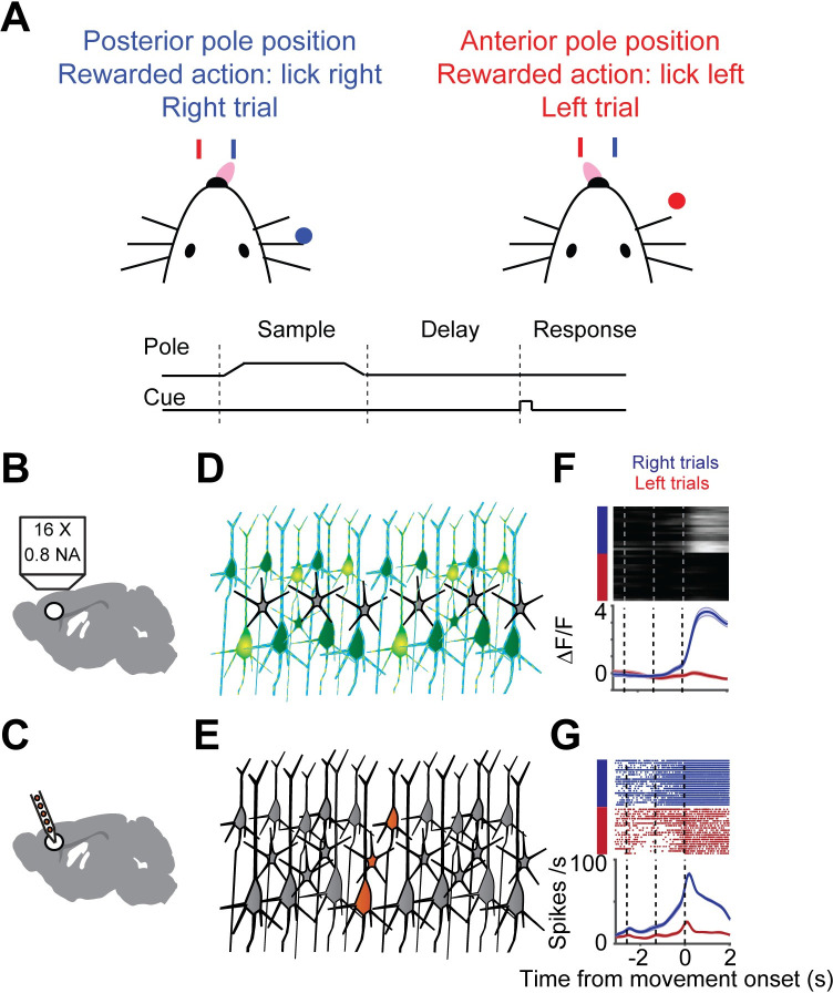
Fig 1
Illustration of sampling population activity in anterior lateral motor cortex using imaging and electrophysiology.
A. Delayed-response, two alternative forced-choice task. Mice discriminated a pole position (anterior or posterior) and reported it by directional licking (lick right, blue; lick left, red) after a de...
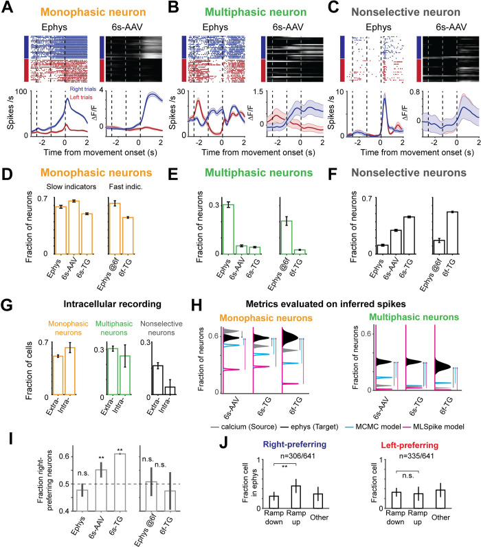
Fig 2
Single neuron trial-type selectivity differs between imaging and ephys.
A. Example neurons with monophasic selectivity. Left, ephys; right, imaging. B , Same as A for multiphasic neurons. C , Same as A for non-selective neurons. D-F , Fraction of selective neurons in dept...
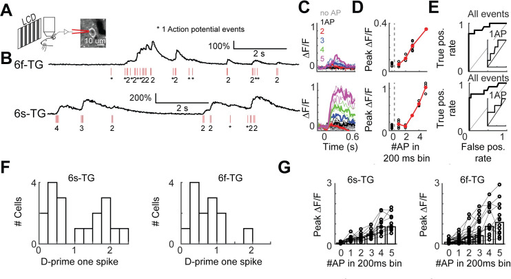
Fig 3
Simultaneous loose-seal recordings and calcium imaging of layer 2/3 pyramidal neurons in vivo .
A. Illustration of the recording setup. Transgenic mice expressing GCaMP6s (GP4.3) or GCaMP6f (GP5.17) were lightly anesthetized and viewed drifting grating visual stimuli. GCaMP-expressing L2/3 neuro...
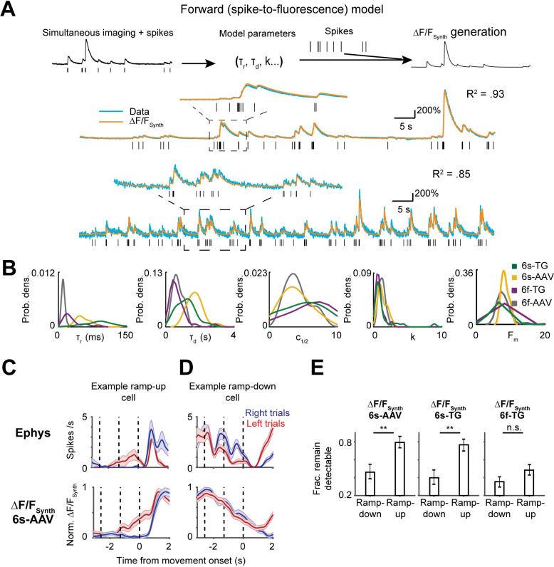
Fig 4
Forward modeling of the spike-to-fluorescence transformation largely explains difference in selectivity patterns.
A. spike-to-fluorescence model. Top: schematic plot of the spike-to-fluorescence (S2F) forward model that generates a synthetic fluorescence trace (u0394F/F Synth ) from an input spike train. Middle: ...
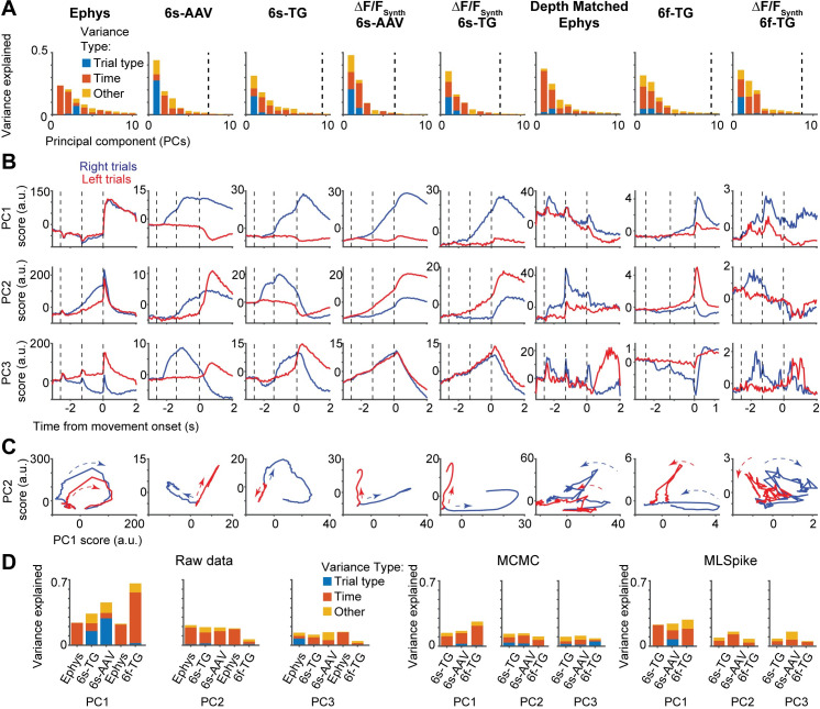
Fig 5
Different sources of variability extracted in dimensionality reduction on imaging and ephys.
A. Fraction of variance of neural activity explained by principal components 1u201310 divided into different sources of variability: red: temporal dynamics; blue: trial type; yellow: other (interactio...
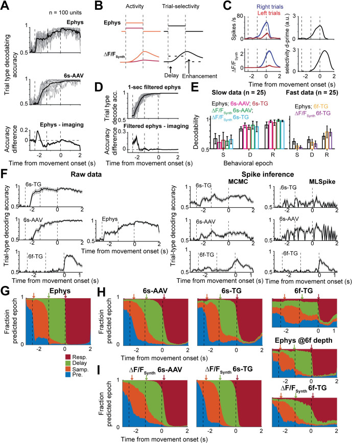
Fig 6
Population decoding differs in sensitivity and temporal profile between imaging and ephys.
A. Performance of instantaneous regularized linear-discriminant-analysis (LDA) trail-type decoder for 100-unit subpopulations. Vertical dotted lines indicate behavioral epochs, from left to right: pre...
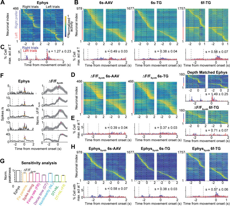
Fig 7
Temporal dispersion of population dynamics differs between imaging and ephys.
A. Heatmap of normalized trial-averaged firing rates for right trials (left) and left trials (right) for ephys data. Firing rates were normalized to maximum of activity across both conditions. Neurons...
Figure images are served from the NIH/NLM PubMed Central Open Access Subset or Europe PMC; copyright remains with the publishers and authors.
💬 Discussion
0 commentsNo comments yet. Be the first to start a discussion!
Leave a Comment