Abstract
During spatial learning, hippocampal (HPC) place maps reorganize to represent new goal locations, but little is known about the circuit mechanisms facilitating these changes. Here, we examined how neuromodulation via locus coeruleus (LC) projections to HPC area CA1 (LC-CA1) regulates the overrepresentation of CA1 place cells near rewarded locations. Using two-photon calcium imaging, we monitored the activity of LC-CA1 fibers in the mouse dorsal HPC. We find that the LC-CA1 projection signals the translocation of a reward, predicting behavioral performance on a goal-oriented spatial learning task. An optogenetic stimulation mimicking this LC-CA1 activity induces place cell reorganization around a familiar reward, while its inhibition decreases the degree of overrepresentation around a translocated reward. Our results show that LC acts in conjunction with other factors to induce goal-directed reorganization of HPC representations and provide a better understanding of the role of neuromodulatory actions on HPC place map plasticity.
🔬 Techniques
💻 Software
✨ Fluorophores
🧪 Sample Preparation
🏭 Microscope Brands
🧪 Reagent Suppliers
📷 Detectors
💻 Software Details
🏛️ Research Organizations (ROR)
Affiliated research institutions:
📋 Methods
LEAD CONTACT AND MATERIALS AVAILABILITY
Further information and requests for resources and reagents should be directed to the Lead Contact Attila Losonczy ( al2856@columbia.edu ). All unique/stable reagents generated in this study are available from the Lead Contact with a completed Materials Transfer Agreement.
EXPERIMENTAL MODEL AND SUBJECT DETAILS
Experiments were conducted in accordance with NIH guidelines and with the approval of the Columbia University Institutional Animal Care and Use Committee. Experiments were conducted with male and female mice, age 2–4 months, on a C57BL/6J background. LC injections were performed in Th-IRES-Cre mice (obtained from Dr. Eric Kandel’s laboratory at Columbia University) ( Lindeberg et al., 2004 ), and Cre-negative littermates or wild-type mice. VIP-IRES-Cre mice were crossed to C57BL/6J mice, and then crossed with Th-IRES-Cre mice, which were on a C57BL/6J background. METHOD DETAILS Viruses Recombinant adeno-associated viruses (rAAVs) were used for GCaMP6 and optogenetic channel expression. Cre-dependent bReaChes ( Rajasethupathy et al., 2015 ), a red-excitation shifted variant of channelrhodopsin, expression was achieved with rAAV2/9:Ef1a-(bReaChes-tdTomato) Cre (obtained from Dr. Boris Zemelman, UT Texas, Austin), GCaMP6s expression in the LC with rAAV 2/9:Ef1a-(GCaMP6s) Cre (Dr. Boris Zemelman, UT Texas, Austin). For expression in CA1PCs, rAAV2/1:hSyn-GCaMP6f and rAAV2/1:CaMKII-GCaMP6f were used (see Key Resources Table ). For experiments with viral mixtures, viruses were mixed in a 1:1 ratio. If animals were used for multiple experiments, they were trained on a burlap belt between paradigms. Viral injection and hippocampal window/headpost implant Viral injections were performed with a Nanoject syringe, as previously described ( Lovett-Barron et al., 2014 ). Briefly, mice were anesthetized with isoflurane and treated with buprenorphine or meloxicam to minimize postoperative discomfort. The skull was exposed and a hole was drilled, and a sterile glass capillary containing viral mixtures was lowered into the brain. After injections, the skin was sutured and mice were allowed to recover. The LC was injected bilaterally at coordinates AP −5.45 mm, ML ±1.28 mm, and DV −3.65 mm with 150 – 300 nL of virus. The dorsal HPC area CA1 was injected in the left hemisphere at coordinates from Bregma AP −2.1 or −2.2, ML −1.5 or −1.75, and DV −1.2, −1.1, and −1.0 with 50–64 nL of virus at each DV site. Mice were implanted with an imaging window (diameter 3.0 mm, height 1.5 mm) over the left dorsal-intermediate hippocampus with a stainless-steel or brass headpost. Imaging cannulas were constructed by adhering (Norland optical adhesive) a 3-mm glass coverslip (64–0720, Warner) to the steel cannula (Ziggy’s tubes and wires). The surgical procedure has been described previously ( Lovett-Barron et al., 2014 ). Briefly, mice were anesthetized and treated with buprenorphine or meloxicam, the skull was exposed and a 3 mm hole was made in the skull. Bone, dura and cortical layers were removed, while flushing with ice-cold cortex buffer. The cannula was inserted into the hole, secured with Vetbond, and a headpost was affixed to the skull with dental cement. Mice recovered in their home cage, and were monitored for three days post-surgery. In vivo calcium two-photon imaging and optogenetics Imaging was conducted using a two-photon 8 kHz resonant scanner (Bruker). A piezoelectric crystal was coupled to the objective as described previously ( Danielson et al., 2016 ) in order to allow fast displacement along the Z-axis. The objective was a Nikon 40x NIR water immersion, 0.8 NA, 3.5 mm working distance. The excitation laser was 920 nm (50–100 mW, Coherent Ultra II). For some structural images in red, the laser was 1070 nm (Coherent Fidelity), and scanning was interlaced with the 920 nm laser for green excitation. Red (tdTomato) and green (GCaMP6) channels were separated by emission cubes as described previously ( Danielson et al., 2016 ). Fluorescence signals were collected using photon multiplier tubes (PMT, GaAsP PMT, Hamamatsu R3896). A preamp (1.4 × 10⁵ dB, Bruker) was used to amplify signals before digitization. Pockels cells were used to regulate the power of the LED reaching the tissue. Images were acquired at 1x digital zoom, 1.2, or 1.4, with 512 × 512 pixels. For CA1PCs, two separate planes were acquired from 20 μm and up to 30 μm apart, with the piezo waiting to settle at each plane for 35ms, such that the frame rate was about 8 Hz. For axons, 2–5 planes 2 μm apart were acquired to maintain the axon in the z plane. For optogenetic experiments, a dichroic mirror was used to allow red light to pass through into the brain, and green light to be reflected into the PMT. The stimulation was performed with an ultrafast and high-power collimated LED, at 625 nm (Prizmatix, 625 nm). It was triggered using an Arduino board that gated the inverse photostimulation signal of the Pockels cell, which turns off briefly between mirror turnaround, as well as when the piezo reverses direction. The average power of the LED was 35–70 mW measured under the objective. This approach allowed us to protect our PMTs from the high intensity illumination but still take the advantage of the fast, full frame resonant galvo scanning without losing frames during photostimulation. Behavioral experiments Mice were trained on a cue-free burlap belt. 3–4 days after the implantation surgery, they were water deprived. First, they were habituated to head fixation for several 10-minute sessions. Then they were allowed to lick freely for water, which was delivered initially at 15 locations on the belt. Then the animals were required to lick initially to receive the water reward, and each day the reward schedule was gradually dropped to 3 rewards per two meter burlap belt. Training took approximately 10 days. During imaging, mice ran on an unfamiliar cued belt, with multiple types of fabric and cues. For CA1PC imaging, we used multisensory cues, including a constant stream of pinene-scented air, a blinking ultraviolet LED, and a constant tone. For the LC imaging, since LC axons are sensitive to multisensory stimuli, and we wanted to examine signals in response to behavioral factors, these additional stimuli were not used. The mice ran three 10-minute sessions per day, separated by at least forty-five minutes. The mice were required to lick initially for the reward, and rewards were available in the location for a maximum of two seconds. For random foraging during CA1PC recordings and LED stimulation, animals were habituated to the belt 3x for 1 day to have maximally stable place fields, then they ran 3 × 10-minute sessions per day for three days. LED stimulation began on the third session of the first imaging day, and continued for 5–6 sessions. Behavioral performance was assessed by the proportion of licks in the area immediately preceding the reward zone, beginning 35 cm before the reward.
Show full methods section
LEAD CONTACT AND MATERIALS AVAILABILITY
Further information and requests for resources and reagents should be directed to the Lead Contact Attila Losonczy ( al2856@columbia.edu ). All unique/stable reagents generated in this study are available from the Lead Contact with a completed Materials Transfer Agreement.
EXPERIMENTAL MODEL AND SUBJECT DETAILS
Experiments were conducted in accordance with NIH guidelines and with the approval of the Columbia University Institutional Animal Care and Use Committee. Experiments were conducted with male and female mice, age 2–4 months, on a C57BL/6J background. LC injections were performed in Th-IRES-Cre mice (obtained from Dr. Eric Kandel’s laboratory at Columbia University) ( Lindeberg et al., 2004 ), and Cre-negative littermates or wild-type mice. VIP-IRES-Cre mice were crossed to C57BL/6J mice, and then crossed with Th-IRES-Cre mice, which were on a C57BL/6J background. METHOD DETAILS Viruses Recombinant adeno-associated viruses (rAAVs) were used for GCaMP6 and optogenetic channel expression. Cre-dependent bReaChes ( Rajasethupathy et al., 2015 ), a red-excitation shifted variant of channelrhodopsin, expression was achieved with rAAV2/9:Ef1a-(bReaChes-tdTomato) Cre (obtained from Dr. Boris Zemelman, UT Texas, Austin), GCaMP6s expression in the LC with rAAV 2/9:Ef1a-(GCaMP6s) Cre (Dr. Boris Zemelman, UT Texas, Austin). For expression in CA1PCs, rAAV2/1:hSyn-GCaMP6f and rAAV2/1:CaMKII-GCaMP6f were used (see Key Resources Table ). For experiments with viral mixtures, viruses were mixed in a 1:1 ratio. If animals were used for multiple experiments, they were trained on a burlap belt between paradigms. Viral injection and hippocampal window/headpost implant Viral injections were performed with a Nanoject syringe, as previously described ( Lovett-Barron et al., 2014 ). Briefly, mice were anesthetized with isoflurane and treated with buprenorphine or meloxicam to minimize postoperative discomfort. The skull was exposed and a hole was drilled, and a sterile glass capillary containing viral mixtures was lowered into the brain. After injections, the skin was sutured and mice were allowed to recover. The LC was injected bilaterally at coordinates AP −5.45 mm, ML ±1.28 mm, and DV −3.65 mm with 150 – 300 nL of virus. The dorsal HPC area CA1 was injected in the left hemisphere at coordinates from Bregma AP −2.1 or −2.2, ML −1.5 or −1.75, and DV −1.2, −1.1, and −1.0 with 50–64 nL of virus at each DV site. Mice were implanted with an imaging window (diameter 3.0 mm, height 1.5 mm) over the left dorsal-intermediate hippocampus with a stainless-steel or brass headpost. Imaging cannulas were constructed by adhering (Norland optical adhesive) a 3-mm glass coverslip (64–0720, Warner) to the steel cannula (Ziggy’s tubes and wires). The surgical procedure has been described previously ( Lovett-Barron et al., 2014 ). Briefly, mice were anesthetized and treated with buprenorphine or meloxicam, the skull was exposed and a 3 mm hole was made in the skull. Bone, dura and cortical layers were removed, while flushing with ice-cold cortex buffer. The cannula was inserted into the hole, secured with Vetbond, and a headpost was affixed to the skull with dental cement. Mice recovered in their home cage, and were monitored for three days post-surgery. In vivo calcium two-photon imaging and optogenetics Imaging was conducted using a two-photon 8 kHz resonant scanner (Bruker). A piezoelectric crystal was coupled to the objective as described previously ( Danielson et al., 2016 ) in order to allow fast displacement along the Z-axis. The objective was a Nikon 40x NIR water immersion, 0.8 NA, 3.5 mm working distance. The excitation laser was 920 nm (50–100 mW, Coherent Ultra II). For some structural images in red, the laser was 1070 nm (Coherent Fidelity), and scanning was interlaced with the 920 nm laser for green excitation. Red (tdTomato) and green (GCaMP6) channels were separated by emission cubes as described previously ( Danielson et al., 2016 ). Fluorescence signals were collected using photon multiplier tubes (PMT, GaAsP PMT, Hamamatsu R3896). A preamp (1.4 × 10⁵ dB, Bruker) was used to amplify signals before digitization. Pockels cells were used to regulate the power of the LED reaching the tissue. Images were acquired at 1x digital zoom, 1.2, or 1.4, with 512 × 512 pixels. For CA1PCs, two separate planes were acquired from 20 μm and up to 30 μm apart, with the piezo waiting to settle at each plane for 35ms, such that the frame rate was about 8 Hz. For axons, 2–5 planes 2 μm apart were acquired to maintain the axon in the z plane. For optogenetic experiments, a dichroic mirror was used to allow red light to pass through into the brain, and green light to be reflected into the PMT. The stimulation was performed with an ultrafast and high-power collimated LED, at 625 nm (Prizmatix, 625 nm). It was triggered using an Arduino board that gated the inverse photostimulation signal of the Pockels cell, which turns off briefly between mirror turnaround, as well as when the piezo reverses direction. The average power of the LED was 35–70 mW measured under the objective. This approach allowed us to protect our PMTs from the high intensity illumination but still take the advantage of the fast, full frame resonant galvo scanning without losing frames during photostimulation. Behavioral experiments Mice were trained on a cue-free burlap belt. 3–4 days after the implantation surgery, they were water deprived. First, they were habituated to head fixation for several 10-minute sessions. Then they were allowed to lick freely for water, which was delivered initially at 15 locations on the belt. Then the animals were required to lick initially to receive the water reward, and each day the reward schedule was gradually dropped to 3 rewards per two meter burlap belt. Training took approximately 10 days. During imaging, mice ran on an unfamiliar cued belt, with multiple types of fabric and cues. For CA1PC imaging, we used multisensory cues, including a constant stream of pinene-scented air, a blinking ultraviolet LED, and a constant tone. For the LC imaging, since LC axons are sensitive to multisensory stimuli, and we wanted to examine signals in response to behavioral factors, these additional stimuli were not used. The mice ran three 10-minute sessions per day, separated by at least forty-five minutes. The mice were required to lick initially for the reward, and rewards were available in the location for a maximum of two seconds. For random foraging during CA1PC recordings and LED stimulation, animals were habituated to the belt 3x for 1 day to have maximally stable place fields, then they ran 3 × 10-minute sessions per day for three days. LED stimulation began on the third session of the first imaging day, and continued for 5–6 sessions. Behavioral performance was assessed by the proportion of licks in the area immediately preceding the reward zone, beginning 35 cm before the reward.
Histology and immunohistochemistry
After the last imaging sessions mice were put under deep isoflurane anesthesia and transcardially perfused with 0.1 M PBS followed by 4% paraformaldehyde in 0.1 M PBS. After overnight post-fixation in the same solution the brains were transferred to PBS. The LC was sliced with a vibratome into 50 μm slices, while the hippocampus was sliced into 50–70 μm slices. Slices were washed 3x with 0.1 M PB, then washed in tris-buffered saline (TBS) with 0.3% triton (TBST) several times, incubated in 10% normal donkey serum in TBS for 45 minutes, then incubated for 1 hour at room temperature and for ~2 days in primary antibodies: slices were incubated with the following antibodies (for details see STAR methods ): anti-GFP, anti-dsRed, or anti-Th (either chicken or rabbit). The slices were then washed with TBS several times and incubated with the appropriate secondary antibodies (see Key Resources Table ). The slices were rinsed, mounted with Aquamount, and imaged on a confocal microscope.
QUANTIFICATION AND STATISTICAL ANALYSIS Calcium imaging data preprocessing
The preprocessing steps for the raw fluorescence signal have been described elsewhere ( Danielson et al., 2016 ). Briefly, the imaging data was motion corrected using the SIMA software package ( Kaifosh et al., 2014 ). Frames where the motion correction failed were discarded if they were below a certain threshold of similarity to the time-averaged image of the entire calcium video. CA1PCs or LC-CA1 axons were hand-segmented using a data visualization server program developed in the lab. The same LC-CA1 axons and CA1PCs were transferred across sessions wherever possible, and identified with a unique ID, so that their activity across sessions could be tracked. Relative fluorescence changes in CA1PCs ( ΔF/F ) were computed with a baseline calculation method adapted from Jia et al.( Jia et al., 2011 ), with uniform smoothing window t 1 = 3s and baseline size t 2 = 60s. For CA1PCs, we detected statistically significant transients as described previously ( Danielson et al., 2016 ) to use for place field calculations. More analyses were implemented using Python using custom written scripts. For axons, the details are located in Figure S1 . We first determined that the axons were synchronous by looking at the mean pairwise correlation coefficient in each session for each ROI (axon segment). A shuffle distribution of pairwise correlation coefficients was generated by taking the same axon at different sessions in time. The 99th percentile of the shuffle distribution constituted the threshold for each animal above which ROIs were included in the analyses. For each session, the remaining axons were simplified as a single trace by taking the first principal component of the signal. We finally removed any linear trends in the resulting trace over chunks of 80s of data (in case the bleaching process occurred exponentially), and smoothed using a Savitzky-Golay filter (sliding window of 21 frames, polynomial degree 6). Place cell metrics Detailed methods for determining statistically significant place cells and their place fields, and the enrichment of the place fields around the reward zone are described ( Danielson et al., 2016 ; Zaremba et al., 2017 ). Briefly, for each CA1PC, calcium transients with onsets during running bouts of at least 1 s in duration were used to calculate the spatial information of the cell ( Skaggs et al., 1993 ). Transients were randomly shuffled to different times during the running events, and the spatial information was recalculated. One thousand iterations were performed to create a null distribution for spatial information, and the cell was considered to be a place cell if its spatial information was above the 95 th percentile of the null distribution. The belt was evenly divided into 100 spatial bins, and the place field was calculated from its transient rate map over these bins. The rate map was the number of transients in a given spatial bin normalized by the animal’s occupancy in that spatial bin, which was then smoothed with a Gaussian kernel (s = 3 spatial bins). To detect individual place fields, each local maximum of the smoothed rate map was fitted with a Gaussian curve centered at that location. For each smoothed rate map, the place fields where the associated Gaussian was smaller than 50% of the largest Gaussian (by measuring the total area under the curve) were discarded. The remaining Gaussians were considered place fields. The centroid of each place field was determined by the location of the peak of the Gaussian, and the location of the centroid of the largest place field was used for enrichment analysis. Enrichment was determined by the proportion of place fields with centroids in the area beginning 25 cm before the reward zone spanning to the end of the zone. The transient frequency was calculated as the rate of significant transients detected by the method described above. The duration of the transient was taken as the beginning and end of the transient, normalized by the frame rate. The amplitude was the peak of the ΔF/F signal. For each statistically significant transient of a place cell, the area under the curve ( Figure S3A ) was computed as the sum of the calcium fluorescence signal during the transient duration, normalized by the frame rate. For Figure S3C , the place cells with place fields outside the reward zone on session 1 were plotted according to the location of their centroids on subsequent sessions. Place fields within the reward zone on session 5 were plotted on previous and subsequent sessions as well. The proportion of place cells inside the reward zone compared with cells outside the reward zone was averaged across sessions before the LED (sessions 1–4, LED off), and across sessions with the LED ( Figure S3D , LED on). Recurrence probability ( Figure S3B ) was calculated by taking the place fields within the reward zone on day 9 in control and experimental groups, and determining the proportion of those cells that were place cells on previous days.
Generalized linear model
We use a generalized linear model to re-generate the calcium activity as a linear function of behavioral variables ( Allen et al., 2017 ; Pinto and Dan, 2015 ; Turi et al., 2019 ). Fitting the GLM coefficients entails finding the linear combination of behavioral covariates which optimally predicts the calcium signal of LC axons. The following behavior variables were used: velocity, licking, and position. All the variables (except position) were smoothed with a Gaussian kernel (σ = 50ms). For the position signal, we divided the treadmill into 100 non-overlapping bins, which were represented in the model by 100 corresponding binary variables that were equal to one during times when the animal occupied that spatial bin and zero otherwise ( Figure S1G ). These behavior variables were fitted to the calcium activity using ridge regression, to manage potential collinearity of predictors and avoid overfitting. For cross-validation, the calcium activity was divided into blocks corresponding to the number of laps in the session. We trained the model on ( n-1 ) laps and then tested on the held-out lap. The testing lap was then rotated to cover all the n laps of the session. Finally, we concatenated all the tested laps to have the cross-validated predicted trace of the entire session. The regularization penalty was optimized separately through cross-validation on the training set, before fitting the final model on the full training set and evaluating prediction quality on the test set. To assess fit quality, we calculated the coefficient of determination (R 2 ) between the model’s predicted axonal calcium activity and the actual axonal calcium activity. To estimate the specific contribution of each category of behavior variables, we also trained a reduced model which contained all variables except the variable of interest. We then calculated the (base-2) log-likelihood ratio between the full model and the reduced model, normalized by the number of time samples, to estimate the information gained (in bits/sample) by including the missing variable. This measure was also estimated only from the held-out test data in the cross-validation procedure. Linear regression between speed and fluorescence signal in LC In order to assess the amplitude of the overshoot of activity seen in the LC signal in the second phase of the goal-oriented task when the animal approaches the reward zone, we looked at the linear relationship between the velocity of the animal and the calcium trace ( Figure 2G ). The rationale behind this analysis is that it is impractical to estimate a baseline to generate ΔF/F values (either static or dynamic) since the activity tracks velocity (as seen in the GLM analysis, Figure 2C ), and differences in ΔF/F are small. The relationship between velocity and the calcium trace was the best measure to detect changes in LC signal without altering or transforming the data to get rid of the velocity component. We computed a linear regression between the two variables in the window −35 to 0 cm before the reward, and extracted the slope of the fit.
Statistics
For all standard statistical tests (statistical details of experiments can be found in the figure legends), the a was chosen to be 0.05 for statistical significance. No statistical methods were used to predetermine sample sizes, but our sample sizes are similar to those reported in previous publications. For all the analyses, if data points followed a normal distribution (confirmed using the Kolmogorov-Smirnov test), depending on the type of comparison, a two-tailed paired sample or unpaired t-test was applied. For non-normal distributions, depending on the type of comparison, the non-parametric two-tailed paired-sample Wilcoxon signed rank test or two-tailed unpaired Mann-Whitney U test was used. If a sample had fewer than five data points, a non-parametric test was used as we did not have enough statistical power to test for normality. *, p < 0.05, **, p < 0.01, ***, p < 0.001. Data analysis and figures were done using custom made software in Python 2.7.15™ ( https://www.python.org/ ).
DATA AND SOFTWARE AVAILABILITY
The data generated in this study and the analyses code will be made available upon reasonable request to the corresponding author.
LEAD CONTACT AND MATERIALS AVAILABILITY
Further information and requests for resources and reagents should be directed to the Lead Contact Attila Losonczy ( al2856@columbia.edu ). All unique/stable reagents generated in this study are available from the Lead Contact with a completed Materials Transfer Agreement.
EXPERIMENTAL MODEL AND SUBJECT DETAILS
Experiments were conducted in accordance with NIH guidelines and with the approval of the Columbia University Institutional Animal Care and Use Committee. Experiments were conducted with male and female mice, age 2–4 months, on a C57BL/6J background. LC injections were performed in Th-IRES-Cre mice (obtained from Dr. Eric Kandel’s laboratory at Columbia University) ( Lindeberg et al., 2004 ), and Cre-negative littermates or wild-type mice. VIP-IRES-Cre mice were crossed to C57BL/6J mice, and then crossed with Th-IRES-Cre mice, which were on a C57BL/6J background.
METHOD DETAILS Viruses Recombinant adeno-associated viruses (rAAVs) were used for GCaMP6 and optogenetic channel expression. Cre-dependent bReaChes ( Rajasethupathy et al., 2015 ), a red-excitation shifted variant of channelrhodopsin, expression was achieved with rAAV2/9:Ef1a-(bReaChes-tdTomato) Cre (obtained from Dr. Boris Zemelman, UT Texas, Austin), GCaMP6s expression in the LC with rAAV 2/9:Ef1a-(GCaMP6s) Cre (Dr. Boris Zemelman, UT Texas, Austin). For expression in CA1PCs, rAAV2/1:hSyn-GCaMP6f and rAAV2/1:CaMKII-GCaMP6f were used (see Key Resources Table ). For experiments with viral mixtures, viruses were mixed in a 1:1 ratio. If animals were used for multiple experiments, they were trained on a burlap belt between paradigms. Viral injection and hippocampal window/headpost implant Viral injections were performed with a Nanoject syringe, as previously described ( Lovett-Barron et al., 2014 ). Briefly, mice were anesthetized with isoflurane and treated with buprenorphine or meloxicam to minimize postoperative discomfort. The skull was exposed and a hole was drilled, and a sterile glass capillary containing viral mixtures was lowered into the brain. After injections, the skin was sutured and mice were allowed to recover. The LC was injected bilaterally at coordinates AP −5.45 mm, ML ±1.28 mm, and DV −3.65 mm with 150 – 300 nL of virus. The dorsal HPC area CA1 was injected in the left hemisphere at coordinates from Bregma AP −2.1 or −2.2, ML −1.5 or −1.75, and DV −1.2, −1.1, and −1.0 with 50–64 nL of virus at each DV site. Mice were implanted with an imaging window (diameter 3.0 mm, height 1.5 mm) over the left dorsal-intermediate hippocampus with a stainless-steel or brass headpost. Imaging cannulas were constructed by adhering (Norland optical adhesive) a 3-mm glass coverslip (64–0720, Warner) to the steel cannula (Ziggy’s tubes and wires). The surgical procedure has been described previously ( Lovett-Barron et al., 2014 ). Briefly, mice were anesthetized and treated with buprenorphine or meloxicam, the skull was exposed and a 3 mm hole was made in the skull. Bone, dura and cortical layers were removed, while flushing with ice-cold cortex buffer. The cannula was inserted into the hole, secured with Vetbond, and a headpost was affixed to the skull with dental cement. Mice recovered in their home cage, and were monitored for three days post-surgery. In vivo calcium two-photon imaging and optogenetics Imaging was conducted using a two-photon 8 kHz resonant scanner (Bruker). A piezoelectric crystal was coupled to the objective as described previously ( Danielson et al., 2016 ) in order to allow fast displacement along the Z-axis. The objective was a Nikon 40x NIR water immersion, 0.8 NA, 3.5 mm working distance. The excitation laser was 920 nm (50–100 mW, Coherent Ultra II). For some structural images in red, the laser was 1070 nm (Coherent Fidelity), and scanning was interlaced with the 920 nm laser for green excitation. Red (tdTomato) and green (GCaMP6) channels were separated by emission cubes as described previously ( Danielson et al., 2016 ). Fluorescence signals were collected using photon multiplier tubes (PMT, GaAsP PMT, Hamamatsu R3896). A preamp (1.4 × 10⁵ dB, Bruker) was used to amplify signals before digitization. Pockels cells were used to regulate the power of the LED reaching the tissue. Images were acquired at 1x digital zoom, 1.2, or 1.4, with 512 × 512 pixels. For CA1PCs, two separate planes were acquired from 20 μm and up to 30 μm apart, with the piezo waiting to settle at each plane for 35ms, such that the frame rate was about 8 Hz. For axons, 2–5 planes 2 μm apart were acquired to maintain the axon in the z plane. For optogenetic experiments, a dichroic mirror was used to allow red light to pass through into the brain, and green light to be reflected into the PMT. The stimulation was performed with an ultrafast and high-power collimated LED, at 625 nm (Prizmatix, 625 nm). It was triggered using an Arduino board that gated the inverse photostimulation signal of the Pockels cell, which turns off briefly between mirror turnaround, as well as when the piezo reverses direction. The average power of the LED was 35–70 mW measured under the objective. This approach allowed us to protect our PMTs from the high intensity illumination but still take the advantage of the fast, full frame resonant galvo scanning without losing frames during photostimulation. Behavioral experiments Mice were trained on a cue-free burlap belt. 3–4 days after the implantation surgery, they were water deprived. First, they were habituated to head fixation for several 10-minute sessions. Then they were allowed to lick freely for water, which was delivered initially at 15 locations on the belt. Then the animals were required to lick initially to receive the water reward, and each day the reward schedule was gradually dropped to 3 rewards per two meter burlap belt. Training took approximately 10 days. During imaging, mice ran on an unfamiliar cued belt, with multiple types of fabric and cues. For CA1PC imaging, we used multisensory cues, including a constant stream of pinene-scented air, a blinking ultraviolet LED, and a constant tone. For the LC imaging, since LC axons are sensitive to multisensory stimuli, and we wanted to examine signals in response to behavioral factors, these additional stimuli were not used. The mice ran three 10-minute sessions per day, separated by at least forty-five minutes. The mice were required to lick initially for the reward, and rewards were available in the location for a maximum of two seconds. For random foraging during CA1PC recordings and LED stimulation, animals were habituated to the belt 3x for 1 day to have maximally stable place fields, then they ran 3 × 10-minute sessions per day for three days. LED stimulation began on the third session of the first imaging day, and continued for 5–6 sessions. Behavioral performance was assessed by the proportion of licks in the area immediately preceding the reward zone, beginning 35 cm before the reward.
Histology and immunohistochemistry
After the last imaging sessions mice were put under deep isoflurane anesthesia and transcardially perfused with 0.1 M PBS followed by 4% paraformaldehyde in 0.1 M PBS. After overnight post-fixation in the same solution the brains were transferred to PBS. The LC was sliced with a vibratome into 50 μm slices, while the hippocampus was sliced into 50–70 μm slices. Slices were washed 3x with 0.1 M PB, then washed in tris-buffered saline (TBS) with 0.3% triton (TBST) several times, incubated in 10% normal donkey serum in TBS for 45 minutes, then incubated for 1 hour at room temperature and for ~2 days in primary antibodies: slices were incubated with the following antibodies (for details see STAR methods ): anti-GFP, anti-dsRed, or anti-Th (either chicken or rabbit). The slices were then washed with TBS several times and incubated with the appropriate secondary antibodies (see Key Resources Table ). The slices were rinsed, mounted with Aquamount, and imaged on a confocal microscope.
Supplementary Material Supplementary material
📊 Figures
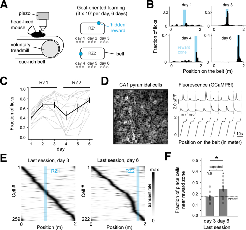
Figure 1.
Place cells are enriched at a translocated reward site during GOL.
A . The goal-oriented learning (GOL) task. Mice searched for an unmarked reward zone (RZ), and water rewards were delivered operantly within the fixed 10cm zone. The RZ was at the same location for 3 ...
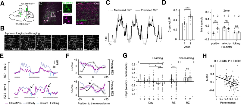
Figure 2.
Locus coeruleus activity changes during GOL
A . Left: LC-CA1 axon labeling strategy. Cre-dependent virus [rAAV2/9:EF1a-(GCaMP6s) Cre ] was injected into the locus coeruleus (LC) of Th-IRES-Cre +/u2212 mice. LC axons in hippocampal (HPC) CA1 wer...
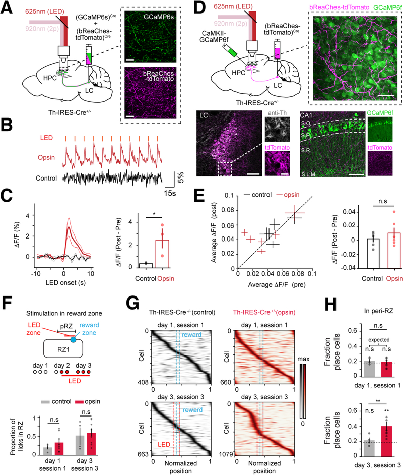
Figure 3.
Stimulating LC-CA1 axons induces CA1 place cell enrichment near a rewarded location during GOL.
A . Left : labelling strategy for optogenetic stimulation and imaging of LC-CA1 axons. The LC was injected with rAAV2/9:EF1a-(GCaMP6s) Cre and rAAV2/9:EF1a-(bReaChes-tdTomato) Cre . Right : time-avera...
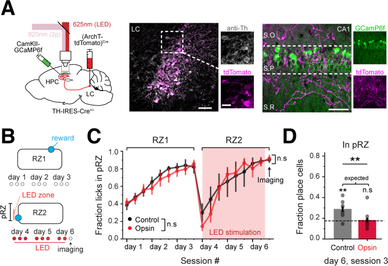
Figure 4.
Inhibition of LC-CA1 axons decreases CA1 place field enrichment
A . Left : labelling strategy for LC-CA1 optogenetic inhibition and imaging of CA1PCs. The LC was injected with rAAV2/9:EF1a-(ArchT-tdTomato) Cre and rAAV2/1:CaMKII-GCaMP6f was injected in CA1. Middle...
Figure images are served from the NIH/NLM PubMed Central Open Access Subset or Europe PMC; copyright remains with the publishers and authors.
💬 Discussion
0 commentsNo comments yet. Be the first to start a discussion!
Leave a Comment