Abstract
Mitotic spindle formation relies on the stochastic capture of microtubules at kinetochores. Kinetochore architecture affects the efficiency and fidelity of this process with large kinetochores expected to accelerate assembly at the expense of accuracy, and smaller kinetochores to suppress errors at the expense of efficiency. We demonstrate that on mitotic entry, kinetochores in cultured human cells form large crescents that subsequently compact into discrete structures on opposite sides of the centromere. This compaction occurs only after the formation of end-on microtubule attachments. Live-cell microscopy reveals that centromere rotation mediated by lateral kinetochore-microtubule interactions precedes the formation of end-on attachments and kinetochore compaction. Computational analyses of kinetochore expansion-compaction in the context of lateral interactions correctly predict experimentally observed spindle assembly times with reasonable error rates. The computational model suggests that larger kinetochores reduce both errors and assembly times, which can explain the robustness of spindle assembly and the functional significance of enlarged kinetochores.
🔬 Techniques
🔭 Microscopes
💻 Software
✨ Fluorophores
🧪 Sample Preparation
🔬 Cell Lines
🏭 Microscope Brands
🧪 Reagent Suppliers
📷 Detectors
💻 Software Details
🏛️ Research Organizations (ROR)
Affiliated research institutions:
📋 Methods
Methods and any associated references are available in the online version of the paper. Note: Supplementary Information is available in the online version of the paper
METHODS Cell Culture, chemical treatments, and live-cell microscopy Human non-transformed hTERT-RPE1 cell line was purchased from Clontech in 2001 at passage number 118.5. Stocks of these cells at passage numbers 120–122 were generated in the Khodjakov lab and kept in liquid nitrogen. A stable clone (RPE1-18), that co-expresses CenpA-eGFP and centrin1-eGFP (both introduced via lentivirus) 47 , was used in most of the experiments described here. Experiments that required visualization of fluorescent Mad2 were conducted in the RPE1 Mad2/Mad2-Venus cell line provided by Dr. Jonathan Pines, University of Cambridge 48 . All cell lines were grown in antibiotic-free DMEM supplemented with 10% FCS (Invitrogen) at 37°C, 5%CO 2 . For live-cell imaging, cells were grown on glass coverslips (#1½) and mounted in Rose chambers containing CO 2 -independent media (Invitrogen) supplemented with 10% FCS. In-house tests for mycoplasma (high-concentration Hoechst staining) are negative. Microtubule depolymerization was induced by nocodazole (Sigma) at 3 μM. Motor activity of CenpE was inhibited with GSK-923295 49 purchased from Haoyuan Chemexpress (Shanghai). Multi-mode 3-D time-lapse recordings were obtained on a Nikon TE-2000E PFS microscope with 100X Plan Apo, N.A. 1.4 oil immersion objective lens. Fluorescence images were captured in a spinning-disc confocal mode (GSU-10, Yokogawa) on a back-illuminated Cascade 512B EM CCD camera (Photometrics). DIC images were recorded on a Photometrics CoolSnap CF camera mounted on a different port of the same microscope. Full 3-D volumes were recorded at each time point at 250-nm Z-steps (48–62 planes depending on cell thickness). To visualize formation of the clear zone we first tracked 3-D positions of mother centrioles and then rotated the 3D volume at each time point to fix position of one mother centriole and orientation of the spindle axis 50 . This processing allowed us to observe chromosome movement in the precisely transverse and axial views. Mother centrioles were tracked FIJI with the standard tracking plugin. 3-D coordinates of the centrioles and the images were then imported into MatLab. The image volume was padded with black (0 value) voxels to prevent cropping during rotation. The rotation was done in two sequential steps, first in XY and then in Z via a custom MatLab script. Rotated and aligned images were transferred back to FIJI. Maximal intensity projections of the entire rotated volume were generated along the spindle axis (transverse view) and orthogonally to the spindle axis (axial view). Each view presented in Fig. 8 contains both centriole pairs and all kinetochores. Incorporation of individual chromosomes into the spindle was observed under conditions that prevented cell rounding during mitosis. A coverslip with 3-μm microfabricated feet was placed on top of the coverslip with the growing cells. The contact between coverslips was maintained with negative pressure using a vacuum pump 51 .
Show full methods section
Methods and any associated references are available in the online version of the paper. Note: Supplementary Information is available in the online version of the paper
METHODS Cell Culture, chemical treatments, and live-cell microscopy Human non-transformed hTERT-RPE1 cell line was purchased from Clontech in 2001 at passage number 118.5. Stocks of these cells at passage numbers 120–122 were generated in the Khodjakov lab and kept in liquid nitrogen. A stable clone (RPE1-18), that co-expresses CenpA-eGFP and centrin1-eGFP (both introduced via lentivirus) 47 , was used in most of the experiments described here. Experiments that required visualization of fluorescent Mad2 were conducted in the RPE1 Mad2/Mad2-Venus cell line provided by Dr. Jonathan Pines, University of Cambridge 48 . All cell lines were grown in antibiotic-free DMEM supplemented with 10% FCS (Invitrogen) at 37°C, 5%CO 2 . For live-cell imaging, cells were grown on glass coverslips (#1½) and mounted in Rose chambers containing CO 2 -independent media (Invitrogen) supplemented with 10% FCS. In-house tests for mycoplasma (high-concentration Hoechst staining) are negative. Microtubule depolymerization was induced by nocodazole (Sigma) at 3 μM. Motor activity of CenpE was inhibited with GSK-923295 49 purchased from Haoyuan Chemexpress (Shanghai). Multi-mode 3-D time-lapse recordings were obtained on a Nikon TE-2000E PFS microscope with 100X Plan Apo, N.A. 1.4 oil immersion objective lens. Fluorescence images were captured in a spinning-disc confocal mode (GSU-10, Yokogawa) on a back-illuminated Cascade 512B EM CCD camera (Photometrics). DIC images were recorded on a Photometrics CoolSnap CF camera mounted on a different port of the same microscope. Full 3-D volumes were recorded at each time point at 250-nm Z-steps (48–62 planes depending on cell thickness). To visualize formation of the clear zone we first tracked 3-D positions of mother centrioles and then rotated the 3D volume at each time point to fix position of one mother centriole and orientation of the spindle axis 50 . This processing allowed us to observe chromosome movement in the precisely transverse and axial views. Mother centrioles were tracked FIJI with the standard tracking plugin. 3-D coordinates of the centrioles and the images were then imported into MatLab. The image volume was padded with black (0 value) voxels to prevent cropping during rotation. The rotation was done in two sequential steps, first in XY and then in Z via a custom MatLab script. Rotated and aligned images were transferred back to FIJI. Maximal intensity projections of the entire rotated volume were generated along the spindle axis (transverse view) and orthogonally to the spindle axis (axial view). Each view presented in Fig. 8 contains both centriole pairs and all kinetochores. Incorporation of individual chromosomes into the spindle was observed under conditions that prevented cell rounding during mitosis. A coverslip with 3-μm microfabricated feet was placed on top of the coverslip with the growing cells. The contact between coverslips was maintained with negative pressure using a vacuum pump 51 .
Fixed-cell immunofluorescence
Cells were pre-extracted in warm PEM buffer (100-mM PIPES, pH 6.9, 2.5-mM EGTA, 5-mM MgCl 2 ) supplemented with 0.5% Triton X-100 for 1 min and fixed with 1%–2% glutaraldehyde for 10 min in PEM. Microtubules were visualized with a monoclonal anti-α-tubulin antibody (DM1a, Sigma; 1:200 dilution). Kinetochores were delineated with the following antibodies: rabbit αCenpF (Novus Biologicals, NB500-101; 1:400 dilution), mouse αCenpE antibody (Abcam, ab5093; 1:200 dilution), mouse αHec1 (Abcam, ab3613; 1:200 dilution), and rabbit αMis12 (kindly provided by Dr. Ian Cheeseman; 1:400 dilution) 52 . Hoechst 33343 (1 μg/ml) was used to stain DNA (chromosomes). Inner kinetochores were visualized via CenpA-GFP fluorescence. Wide-field images were recorded on a DeltaVision imaging system (Applied Precision) with a 100X NA1.35 lens (Olympus). The images were captured with a CH-350 CCD camera (Photometrics) at a 69-nm X-Y pixel size and 200-nm Z-steps. All images were deconvolved with the SoftWoRx 5.0 deconvolution software (Applied Precision) and objective lens-specific point spread functions.
Amira software
(FEI) was used for surface rendering. Segmentation threshold for fluorescence images ( Fig. S2 ) was set at 25% of maximal intensity for each dataset.
Quantification of fluorescence intensity and kinetochore volume
All measurements were conducted in ImageJ/FIJI and calculations - in MS Excel. Integrated fluorescence intensity was measured within a 3-D volume centred on a single kinetochore (whenever possible) or a small group of kinetochores (if their individual signals were not fully resolvable). The dimensions of the volume were set individually to include the entire object of interest (300–2500 voxels, 10×10×3 – 25×25×4 volumes). Background intensity for each measurement was measured in the same-dimensions volume positioned as close as possible to the object of interest. Kinetochore intensity was calculated by subtracting background intensity and dividing the result by the number of kinetochores in the volume. Intensities of multiple kinetochores (usually ~20) were measured in each cell. Mean fluorescence intensity per kinetochore was calculated for individual cells and then the mean value of per-cell averages was calculated. Alternatively, all kinetochores measured under a particular experimental condition were pooled together and the mean value was calculated for this pooled population. Results of both calculations are presented in the figures (Ks = total number of kinetochores; Cs = total number of cells). All values are normalized so that the mean intensity at NEB equals to 1. Kinetochore volumes were measured via “3D Object Counter” routine included in the standard distribution of FIJI. As the amount of CenpF and Mis12 remains constant during late prophase-prometaphase, relative volumes occupied by kinetochores can be segmented at a constant threshold. Threshold values for segmentation were set at 20% of maximal signal intensity for CenpF and 25% for Hec1 datasets. These thresholds were empirically determined to yield maximal numbers of kinetochores per cell with minimal contamination by false objects after segmentation. As in intensity calculations, both mean values were calculated for per cell averages and for the pooled populations (both values are presented in the Figures). All values are normalized so that the mean volume at NEB equals to 1. Mean values were compared in two-tailed Student’s test.
Correlative Electron Microscopy
Cells were fixed in 2.5% glutaraldehyde (Sigma) in PBS (pH 7.4–7.6). Differential interference contrast and fluorescence images were acquired at 0.2-μm Z steps through the entire cell volume shortly after fixation. Post-fixation, embedding, and sectioning were done as previously described 53 . Serial 80-nm thin sections were imaged at 80 kV on either a Zeiss 910 (Carl Zeiss) or JEOL 1400. Correlation of conspicuous morphological features between differential interference contrast and EM images was used to match the orientation and Z positions for individual focal planes and determine exact kinetochore positions.
Computational modelling Microtubule dynamics during spindle assembly
We consider that spindle assembly takes place in the spherical volume that was occupied by the nucleus prior to NEB. Implicitly, we assume, following Wollman and coworkers (2005), that the RanGTP gradient focuses the MTs into the nuclear sphere. This accelerates the search a few-fold but has no effect on the error rate. Two centrosomes are placed at the opposite poles of the sphere at −R cell and +R cell positions. Each centrosome nucleates N MT microtubules that search the space isotropically. Each microtubule is represented by a rod with zero thickness that undergoes dynamic instability. The plus end of a microtubule grows steadily until a catastrophe occurs leading to microtubule shortening. The frequency of catastrophe, as well as the growth and shrinkage rates, is constant (the search with zero and small finite stochastic catastrophe frequencies have been tested and the results were not sensitive to this variation of the model). We use the optimal zero rescue frequency 54 . Microtubule dynamics are simulated by the Monte Carlo algorithm: a random number is generated between 0 and 1 with equal probability. At each computational step (with time increment Δt = 1 sec) the microtubule switches to shortening if this random number is less than [1−exp(−f cat Δt)]. New microtubules grow in random directions and do not turn. In all cases, if a microtubule plus end extends beyond the nuclear sphere’s boundary or encounters a chromosome arm, this microtubule undergoes catastrophe and shrinks all the way back to the centrosome. The values for the number of microtubules generated by each centrosome [N MT ] and the four parameters of dynamic instability [v g , v s , f cat , f res ] used in the simulations are presented in Supplementary Table 1 . The radius of the nuclear/spindle sphere is set to match the geometry of mitosis in RPE1 cells 47 . Effects of the microtubule dynamic instability parameters have been previously explored and discussed 54 . In the current simulations, conservative values from the range explored in reference 54 are used for v g and v s . The number of microtubules in the current simulations (600) is approximately twofold higher than in previous models (250) 54 . This change is introduced to account for the difference in spindle assembly time between HT-29 (15 min 54 ) and RPE1 (8 min 47 ) cells. The model indeed predicts slower absolute assembly time if the number of microtubules is lowered. However, the differences between the predictions in the three considered scenarios (see below) are not affected by the number of microtubules: relative differences in the assembly time as well as the predicted number of errors remain the same. Nascent spindle A second set of stable microtubules runs along the spindle axis and overlaps in the central part of the spindle. Based on microscopy data this dense microtubule array forms shortly after NEB (1–2 min) and persists through prometaphase 47 . The centromeres become positioned on the surface of the nascent spindle shortly (~2 min) after NEB ( Fig. 7 and ref. 45 ) and laterally interact with microtubule walls. In contrast to end-on attachments, lateral interactions can occur along the entire length of microtubule and there is no evidence that these interactions require microtubules to undergo plus-end dynamic instability. Therefore, the nascent spindle in our simulations comprises stable microtubules whose plus ends do not contribute to capture. Geometry of the nascent spindle is derived from previously published data 47 . Microtubule capture A microtubule plus end is instantly captured and stabilized upon encountering a kinetochore. Upon capture, a new dynamic microtubule is nucleated at the same pole to replace the stabilized one. Chromosomes and kinetochores Chromosomes are modelled as solid 3-D cylinders with R CH radius and I ch length ( Supplementary Table 1 ). The initial distribution of chromosomes in the nuclear sphere and their orientation are random. Prior to capture, sister kinetochores are modelled as crescent-shaped objects (see Supplementary Table 1 and Figure S3 for dimensions) wrapped around the central part (equator) of the chromosome. The width w KT and length h KT of kinetochores are kept constant. Upon capturing a microtubule, the kinetochore crescent condenses into a small cylindrical object in τ comp time. This kinetochore geometry reflects our experimental observations ( Figures 1 – 4 ). To complete computations with a reasonable time and avoid difficulty in tracking steric inter-chromosomal interactions, single chromosomes positioned at a fixed distance away from the pole-pole axis are considered in individual simulations. The simulations are then repeated for multiple chromosome positions and random orientations. To obtain the average value of the capture time (τ capt ), we multiplied the capture time of a single chromosome by the logarithm of the total number of chromosomes N CH ( Supplementary Table 1 ).
Tested models
Four different scenarios are considered: Completely random distribution and orientation of chromosomes and kinetochores that remain unaltered upon microtubule capture. Kinetochores are shaped as crescents at the onset of spindle assembly and compact from crescents to discs in τ comp after capture. Microtubule capture leads to rotation of the chromosome and alignment of the centromere axis (line connecting centres of sister kinetochores) along the captured microtubule in time τ rot . Kinetochores are shaped as crescents at the onset of spindle assembly and compact from crescents to discs in τ comp after capture. Because the chromosome arms are largely normal to the pole-pole axis, the rotation primarily occurs around their longitudinal axis. Rapid lateral interactions with the stable microtubules of nascent spindle result in a rapid decrease of the angle between the centromere axis and spindle axis (line connecting the centrosomes) in time τ rot . The angle of chromosome rotation is limited by the ability of kinetochores to maintain direct contact with stable microtubules, which in turn depends on the size of the kinetochore crescent. Kinetochores are shaped as crescents at the onset of spindle assembly and compact from crescents to discs in τ comp after capture. Compaction initiates only after end-on microtubule capture and completes in τ comp . At the beginning of the search, the crescents are small, with the initial gap size of 0.76 μm. In the next 30 s, the crescents grow linearly so that the gap decreases to its final size (0.01 to 0.76 μm in various simulations). The time of crescent growth is constant, irrespective of the final gap size. Lateral interactions decrease the angle between the centromere axis and the spindle axis as in scenario iii; respective rate of rotation is very fast, a few seconds, in this case. Then, the end-on microtubule capture leads to additional rotation of the chromosome and alignment of the centromere axis (line connecting centres of sister kinetochores) along the captured microtubule in time τ rot . Kinetochores compact from crescents to discs in τ comp after end-on microtubule capture. In the most simplistic simulations (scenario i), microtubule capture is not expected to change the position or orientation of the chromosome 55 – 57 . Rotation of the centromere considered in scenarios (ii) 54 and (iii) inevitably shifts the chromosome from its original position. However, in 80% of the cases the mean value of the displacement caused by the brief rapid movement during the initial interaction between kinetochores and microtubules is
📊 Figures
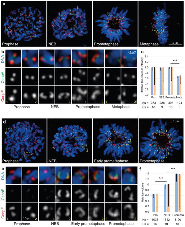
Figure 1
Changes in the outer kinetochore architecture at various stages of mitosis
(au2013c) The outer layer enlarges at the onset of spindle assembly and subsequently downsizes. (a) Maximal intensity projections (include all kinetochores) depicting RPE1 cells at various stages of m...
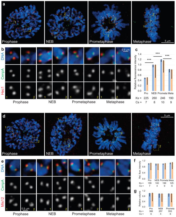
Figure 2
The kinetochore core remains relatively compact throughout mitosis
(a,d) Maximal intensity projections (include all kinetochores) depicting RPE1 cells at various stages of mitosis. (b,e) Examples of individual kinetochores from the boxed areas in (a) and (d) shown at...
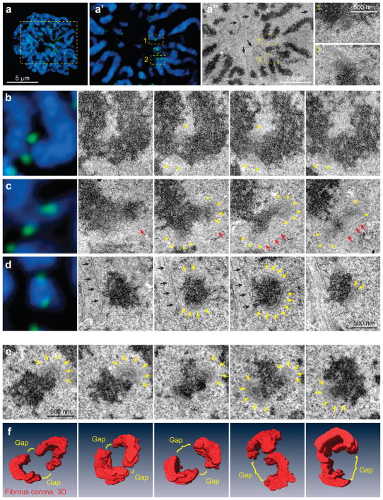
Figure 3
Kinetochore morphology at the onset of spindle assembly
(a) Correlative LM/EM analysis of kinetochore morphology at NEB. Maximal intensity projection of the entire cell and an individual focal plane are shown. Via correlation of LM (au2032) and EM (au2033)...
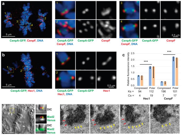
Figure 4
Kinetochore outer layer compaction occurs upon the formation of end-on microtubule attachments
(a,b) Kinetochores are enlarged on polar, but compact on congressed, chromosomes. Whole-cell images are maximal-intensity projections that include all kinetochores in the cell. Individual kinetochores...
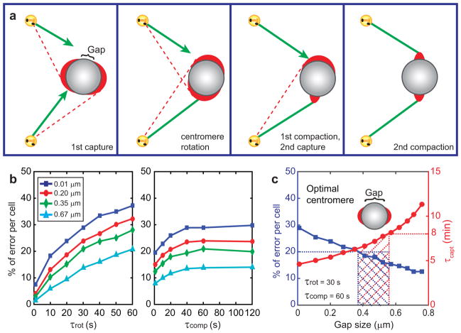
Figure 5
Effects of kinetochore enlargement-compaction on the efficiency and fidelity of capture-driven spindle assembly
(a) Cartoon of the events envisioned in this model. Kinetochores are shown as red crescents. Green lines represent properly attached microtubules, red lines - potential erroneous attachments. (b) Erro...
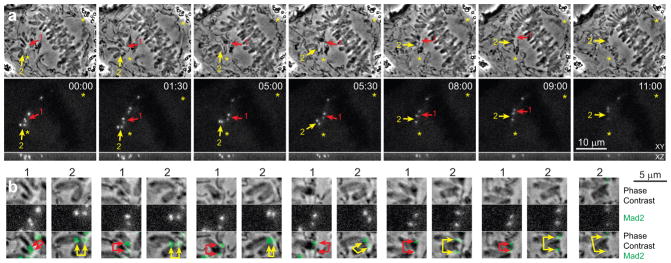
Figure 6
Centromere rotation on the surface of the spindle precedes formation of end-on microtubule attachment
(a) Selected frames from a multi-mode time-lapse recording of a RPE1 cell flattened to 3-u03bcm (See Supplementary Video 1 for full recording). Top row shows phase contrast (medial slice) and the bott...
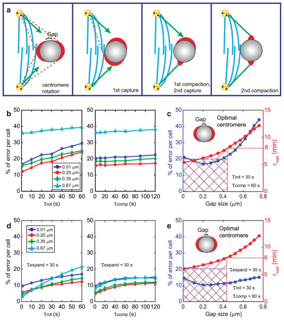
Figure 7
Computational models that consider centromere rotation due to lateral interactions with microtubules predict experimentally-observed parameters of spindle assembly
(a) Cartoon of the events envisioned in the model. Blue lines represent the central part of the nascent spindle with high density of microtubules and devoid of chromosomes. Kinetochores can glide alon...
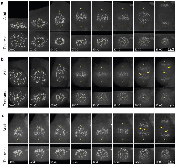
Figure 8
Abnormal geometry of the nascent spindle during early prometaphase correlates with erroneous chromosome segregation
(a) Typical pattern of spindle formation (RPE1 cell). Notice that all centromeres (CenpA-GFP) reside on the surface of the nascent spindle for the first 6u20138 min of prometaphase. (b) Example of an ...
Figure images are served from the NIH/NLM PubMed Central Open Access Subset or Europe PMC; copyright remains with the publishers and authors.
💬 Discussion
0 commentsNo comments yet. Be the first to start a discussion!
Leave a Comment