Abstract
ABSTRACT The cellular morphology and sub-cellular spatial structure critically influence the function of microbial cells. Similarly, the spatial arrangement of genotypes and phenotypes in microbial communities has important consequences for cooperation, competition, and community functions. Fluorescence microscopy techniques are widely used to measure spatial structure inside living cells and communities, which often results in large numbers of images that are difficult or impossible to analyze manually. The rapidly evolving progress in computational image analysis has recently enabled the quantification of a large number of properties of single cells and communities, based on traditional analysis techniques and convolutional neural networks. Here, we provide a brief introduction to core concepts of automated image processing, recent software tools and how to validate image analysis results. We also discuss recent advances in image analysis of microbial cells and communities, and how these advances open up opportunities for quantitative studies of spatiotemporal processes in microbiology, based on image cytometry and adaptive microscope control.
🔬 Techniques
💻 Code & Software
Version 3 of Python mother machine analysis code
Beta release of mother machine analysis framework
MoMA - the MotherMachine Analyzer
ZeroCostDL4Mic: A Google Colab based no-cost toolbox to explore Deep-Learning in Microscopy
💾 Data Repositories
🏛️ Research Organizations (ROR)
Affiliated research institutions:
📋 Methods
Traditional methods for microbial object detection
To understand the approach on which computational object detection in images is built, it is important to appreciate some basic properties of images. Highly sensitive scientific cameras (or point-scanning confocal microscopes) typically acquire two-dimensional (2D) digital grayscale images—one such 2D image is acquired for each channel and/or imaging plane. A 2D image is simply a 2D array (or ‘matrix’) of numbers representing the intensity values of each pixel. The detection of objects in images is then generally based on mathematical operations on this matrix (Gonzalez and Woods 2018 ). A basic mathematical operation in image analysis is the convolution of the image matrix with a kernel, referred to as filtering. When filtering, each pixel of the image is modified based on its neighborhood, resulting in a new image. For example, noise in images can be reduced by averaging pixels over their local neighborhood, resulting in a slightly blurred image. Other choices and combinations of kernels may lead to filters that sharpen the image, emphasize edges, or amplify the signal of structures that have a particular size (e.g. the cell size) to facilitate object detection (Gonzalez and Woods 2018 ). In traditional image analysis, images are typically processed by consecutively applying several different filters to achieve a background removal, an enhancement of the signal-to-noise level, and emphasis of structures of interest (illustrated in Fig. 1 ). Although kernel sizes can be automatically set based on the size of the cells (or colonies) that should be analyzed, the choice and order of filters is ultimately guided by the experience of the person who develops the code. If the quality or structure of the input images are changed, the parameters and filters often need to be adapted. To achieve a semantic segmentation that separates the objects of interest from the background, a threshold is then typically applied to images that have previously undergone filtering, resulting in a binary image termed ‘mask’, which only contains values of 1 and 0 for the foreground and background respectively (Fig. 1 ). A series of morphological operations can then be applied to the binary image so that the mask image represents an accurate semantic segmentation. These morphological operations can for example be the removal of small objects, filling of objects with holes, and widening or narrowing objects, resulting in the final semantic segmentation (Srisha and Khan 2013 ). When individual cells can be visually discerned in images, it is possible to qualitatively pass judgment on the accuracy of the semantic segmentation by comparing the segmentation result with the input image. Such qualitative judgements reach their limit when individual cells cannot be visually distinguished due to crowding or lack of resolution. For example, when measuring the biovolume of a microbial community such as a biofilm without single-cell resolution, the pixel location of the biofilm edge is not uniquely defined, as the biofilm edge is typically characterized by a fluorescence signal gradient that spans several cell diameters. Different segmentation algorithms will therefore identify the biofilm edge to be at slightly different locations. As images of microbial communities without single-cell resolution are commonly analyzed in biofilm research, the need for accurate semantic segmentation has led to a remarkable number of different algorithmic solutions for biofilm biovolume detection (Heydorn et al . 2000 ; Yang et al . 2001 ; Beyenal et al . 2004 ; Yerly et al . 2007 ; Renslow, Lewandowski and Beyenal 2011 ; Klinger-Strobel et al . 2016 ). As illustrated by the development of so many solutions to a problem, traditional semantic segmentation provides users with a lot of freedom in terms of the filters, thresholding and morphological operations, which each come with a set of parameters that can be tuned. A systematic comparison of the accuracy of segmentation results based on quantitative metrics is therefore needed for any image analysis workflow, as described in Box 3 . Following semantic segmentation with traditional computational techniques as outlined above, further processing needs to be applied to achieve an accurate instance segmentation result (Fig. 1 ). Traditional instance segmentation typically relies on different types of edge detection algorithms (Roberts 1965 ; Canny 1986 ; Sobel 2014 ), the watershed algorithm (Beucher and Meyer 1993 ), skeleton algorithm (Lee, Kashyap and Chu 1994 ), or any other operation that works for a particular type of image. Traditional instance segmentation forms the basis of most current image analysis tools for microbiology (Box 1 ), including currently popular tools for bacterial cell biology in 2D images (Ducret, Quardokus and Brun 2016 ; Paintdakhi et al . 2016 ), and for 3D images of bacterial biofilm communities (Drescher et al . 2016 ; Yan et al . 2016 ; Wang et al . 2017 ; Hartmann et al . 2019 ). Traditional image processing approaches can provide accurate results for semantic and instance segmentation, but they have substantial limitations. Usually the selection and order of filters that are applied, the filter parameters, as well as the thresholding and morphological operations have to be adapted in cases when the cells are close together or even touching each other. Similarly, input images that differ in terms of signal-to-noise levels, cell sizes, image background, or distribution of cell sizes, require the analysis algorithms to be adapted, limiting their range of applicability without manual parameter adjustments.
Show full methods section
Traditional methods for microbial object detection
To understand the approach on which computational object detection in images is built, it is important to appreciate some basic properties of images. Highly sensitive scientific cameras (or point-scanning confocal microscopes) typically acquire two-dimensional (2D) digital grayscale images—one such 2D image is acquired for each channel and/or imaging plane. A 2D image is simply a 2D array (or ‘matrix’) of numbers representing the intensity values of each pixel. The detection of objects in images is then generally based on mathematical operations on this matrix (Gonzalez and Woods 2018 ). A basic mathematical operation in image analysis is the convolution of the image matrix with a kernel, referred to as filtering. When filtering, each pixel of the image is modified based on its neighborhood, resulting in a new image. For example, noise in images can be reduced by averaging pixels over their local neighborhood, resulting in a slightly blurred image. Other choices and combinations of kernels may lead to filters that sharpen the image, emphasize edges, or amplify the signal of structures that have a particular size (e.g. the cell size) to facilitate object detection (Gonzalez and Woods 2018 ). In traditional image analysis, images are typically processed by consecutively applying several different filters to achieve a background removal, an enhancement of the signal-to-noise level, and emphasis of structures of interest (illustrated in Fig. 1 ). Although kernel sizes can be automatically set based on the size of the cells (or colonies) that should be analyzed, the choice and order of filters is ultimately guided by the experience of the person who develops the code. If the quality or structure of the input images are changed, the parameters and filters often need to be adapted. To achieve a semantic segmentation that separates the objects of interest from the background, a threshold is then typically applied to images that have previously undergone filtering, resulting in a binary image termed ‘mask’, which only contains values of 1 and 0 for the foreground and background respectively (Fig. 1 ). A series of morphological operations can then be applied to the binary image so that the mask image represents an accurate semantic segmentation. These morphological operations can for example be the removal of small objects, filling of objects with holes, and widening or narrowing objects, resulting in the final semantic segmentation (Srisha and Khan 2013 ). When individual cells can be visually discerned in images, it is possible to qualitatively pass judgment on the accuracy of the semantic segmentation by comparing the segmentation result with the input image. Such qualitative judgements reach their limit when individual cells cannot be visually distinguished due to crowding or lack of resolution. For example, when measuring the biovolume of a microbial community such as a biofilm without single-cell resolution, the pixel location of the biofilm edge is not uniquely defined, as the biofilm edge is typically characterized by a fluorescence signal gradient that spans several cell diameters. Different segmentation algorithms will therefore identify the biofilm edge to be at slightly different locations. As images of microbial communities without single-cell resolution are commonly analyzed in biofilm research, the need for accurate semantic segmentation has led to a remarkable number of different algorithmic solutions for biofilm biovolume detection (Heydorn et al . 2000 ; Yang et al . 2001 ; Beyenal et al . 2004 ; Yerly et al . 2007 ; Renslow, Lewandowski and Beyenal 2011 ; Klinger-Strobel et al . 2016 ). As illustrated by the development of so many solutions to a problem, traditional semantic segmentation provides users with a lot of freedom in terms of the filters, thresholding and morphological operations, which each come with a set of parameters that can be tuned. A systematic comparison of the accuracy of segmentation results based on quantitative metrics is therefore needed for any image analysis workflow, as described in Box 3 . Following semantic segmentation with traditional computational techniques as outlined above, further processing needs to be applied to achieve an accurate instance segmentation result (Fig. 1 ). Traditional instance segmentation typically relies on different types of edge detection algorithms (Roberts 1965 ; Canny 1986 ; Sobel 2014 ), the watershed algorithm (Beucher and Meyer 1993 ), skeleton algorithm (Lee, Kashyap and Chu 1994 ), or any other operation that works for a particular type of image. Traditional instance segmentation forms the basis of most current image analysis tools for microbiology (Box 1 ), including currently popular tools for bacterial cell biology in 2D images (Ducret, Quardokus and Brun 2016 ; Paintdakhi et al . 2016 ), and for 3D images of bacterial biofilm communities (Drescher et al . 2016 ; Yan et al . 2016 ; Wang et al . 2017 ; Hartmann et al . 2019 ). Traditional image processing approaches can provide accurate results for semantic and instance segmentation, but they have substantial limitations. Usually the selection and order of filters that are applied, the filter parameters, as well as the thresholding and morphological operations have to be adapted in cases when the cells are close together or even touching each other. Similarly, input images that differ in terms of signal-to-noise levels, cell sizes, image background, or distribution of cell sizes, require the analysis algorithms to be adapted, limiting their range of applicability without manual parameter adjustments.
📊 Figures
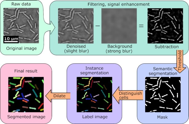
Figure 1.
Typical segmentation workflow in traditional image analysis . A combination of filters, thresholding and morphological operations is applied to the original image (showing Bacillus subtilis cells on a...
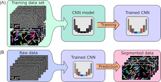
Figure 2.
Typical segmentation workflow using convolutional neural networks . (A) , A set of training data consisting of pairs of raw images and annotated images is used to train a convolutional neural network ...
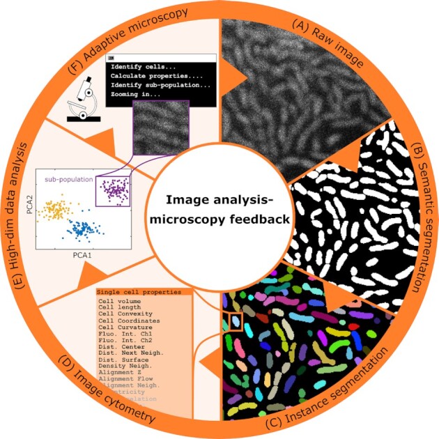
Figure 3.
Integration of single-cell image analysis with adaptive microscopy enables highly specific imaging of communities . After capturing the raw image ( panel A ), cells are distinguished from background t...
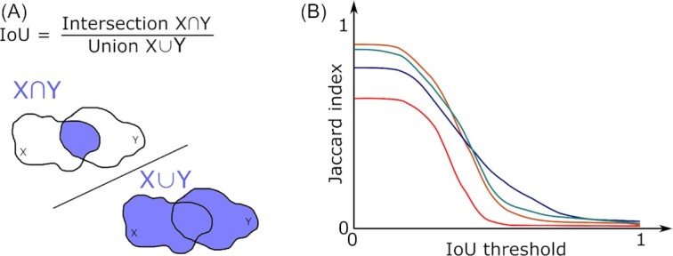
Figure 4.
Schematic figure of the intersection over union (IoU) and the segmentation accuracy for different image analysis methods, measured as a function of the IoU threshold . (A) , Visualization of the IoU, ...
Figure images are served from the NIH/NLM PubMed Central Open Access Subset or Europe PMC; copyright remains with the publishers and authors.
💬 Discussion
0 commentsNo comments yet. Be the first to start a discussion!
Leave a Comment