Abstract
The hypothalamus regulates innate social behaviors, including mating and aggression. These behaviors can be evoked by optogenetic stimulation of specific neuronal subpopulations within MPOA and VMHvl, respectively. Here, we perform dynamical systems modeling of population neuronal activity in these nuclei during social behaviors. In VMHvl, unsupervised analysis identified a dominant dimension of neural activity with a large time constant (>50 s), generating an approximate line attractor in neural state space. Progression of the neural trajectory along this attractor was correlated with an escalation of agonistic behavior, suggesting that it may encode a scalable state of aggressiveness. Consistent with this, individual differences in the magnitude of the integration dimension time constant were strongly correlated with differences in aggressiveness. In contrast, approximate line attractors were not observed in MPOA during mating; instead, neurons with fast dynamics were tuned to specific actions. Thus, different hypothalamic nuclei employ distinct neural population codes to represent similar social behaviors.
🔬 Techniques
🧬 Organisms
✨ Fluorophores
🔬 Cell Lines
💻 Software Details
💻 Code & Software
📂💾 Data Repositories
🏛️ Research Organizations (ROR)
Affiliated research institutions:
📋 Methods
Resource Availability Lead Contact Requests for resources and reagents should be addressed to lead contact, David J. Anderson ( wuwei@caltech.edu ).
Materials availability
This study did not generate new unique reagents.
Data and code availability
Source data used in this paper will be shared by the lead contact upon request. Code used for analyses in this paper is available in the following repositories: https://github.com/lindermanlab/ssm https://github.com/DJALab/VMHvl_MPOA_dynamics Any additional information required to reanalyze the data reported in this paper is available from the lead contact upon request.
Experimental model and subject details Neural imaging data
(Karigo et al., 2021, Remedios et al., 2017, Yang and Anderson, 2022) We analyzed data from three sets of previous experiments 29 , 31 , 39 All experiments were approved by the Institute Animal Care and Use Committee (IACUC) and the Institute Biosafety Committee (IBC) at the California Institute of Technology (Caltech). All experiments utilized heterozygous Esr1 cre/+ knock-in mice on a C457BL6/N background (B6N.129S6(Cg)- Esr1 tm1.1(cre)And I J, JAX strain #017911).
Expression of GCaMP6s
(Remedios et al., 2017, Karigo et al., 2021) or GCaMP7f (Yang et al. 2022) was achieved by stereotaxic injection of a Cre-dependent GCaMP-expressing adeno-associated viruses (AAVs). Briefly, for data obtained from Karigo et al., 2021, mice expressing GCaMP6s selectively in Esr1 neurons in either the medial preoptic area (MPOA) or the ventrolateral subdivision of the ventromedial hypothalamus (VMHvl), were allowed to interact with BALB/c male and female intruders in a standard resident intruder assay (Karigo et al., 2021). Male or female intruders were introduced into the home cage in a random order, with a 5–10 min interval between intruder session. Each session typically lasted 10–20 minutes. Behavior videos of interacting animals were annotated using a custom MATLAB-based interface. A total of 7 behaviors including sniffing, dominance-mount, attack, mount, intromission, interact (periods where animals were close to each other but other behaviors were absent) were annotated with male and female intruders. A head-mounted micro-endoscope (Inscopix, Inc.) was used to acquire Ca 2+ imaging data at 15Hz from either MPOA Esr1 neurons (total of 583 neurons from 3 mice) or VMHvl Esr1 neurons (total of 421 neurons from 3 mice) for neural data analysis described in sections below. For data obtained from Yang et al., 2022, Esr1-Cre mice in which GCaMP7f was expressed selectively in Esr1 neurons in VMHvl, were allowed to interact with BALB/c male intruders in a standard resident intruder assay. In addition to the behaviors annotated for above, male intruders were also “dangled”, where the ano-genital region of the dangled intruder is held next to the resident mouse. A head-mounted micro-endoscope was used to acquire Ca 2+ imaging data at 30Hz from VMHvl Esr1 neurons (386 neurons from 3 mice) for neural data analysis described in sections below. For data obtained from Remedios et al, 2017, Esr1-Cre mice in which GCaMP6s was expressed selectively in Esr1 neurons in VMHvl were allowed to interact with BALB/c male intruders in a standard resident intruder assay. A head-mounted micro-endoscope was used to acquire Ca 2+ imaging data at 30Hz from VMHvl Esr1 neurons (358 neurons from 3 mice) for neural data analysis described in sections below. rSLDS models were fit to data from n=14 mice to extract the time constant of the integration dimension used for correlation with individual differences in aggressiveness in Figure 3O . However 8 of those mice were excluded from decoder analysis of sniffing, mounting and attack, either because they were highly aggressive and attacked without any prior sniffing or dominance mounting (5 mice), or because they were non-aggressive and failed to attack (3 mice). Typically 20–25% of male mice from the C57BL6 background fail to show aggression in resident-intruder assays (Stagkourakis et al., 2020). Method Details Tuning rasters for single neurons We examined the tuning properties of single neurons in VMHvl Esr1 or MPOA Esr1 by creating behavior tuning rasters ( Figure 1 C , D ). We first computed the mean activity of each neuron for each of the 14 manually annotated behavioral actions. To group neurons, we created a set of 40 regressors representing combinations of behavioral actions, and grouped neurons by which single regressor captured the most variance in each cell’s activity. In addition to regressors for individual behaviors, example regressors include signals such as all male-directed actions, all female-directed actions, all male-directed/female-directed/sex-invariant investigative behaviors, and all male-directed/female-directed/sex-invariant consummatory behaviors. Neurons for which no single regressor captured at least 50% of variance in behavior-averaged activity were omitted from the visualization (approximately 5% of cells.)
Show full methods section
Resource Availability Lead Contact Requests for resources and reagents should be addressed to lead contact, David J. Anderson ( wuwei@caltech.edu ).
Materials availability
This study did not generate new unique reagents.
Data and code availability
Source data used in this paper will be shared by the lead contact upon request. Code used for analyses in this paper is available in the following repositories: https://github.com/lindermanlab/ssm https://github.com/DJALab/VMHvl_MPOA_dynamics Any additional information required to reanalyze the data reported in this paper is available from the lead contact upon request.
Experimental model and subject details Neural imaging data
(Karigo et al., 2021, Remedios et al., 2017, Yang and Anderson, 2022) We analyzed data from three sets of previous experiments 29 , 31 , 39 All experiments were approved by the Institute Animal Care and Use Committee (IACUC) and the Institute Biosafety Committee (IBC) at the California Institute of Technology (Caltech). All experiments utilized heterozygous Esr1 cre/+ knock-in mice on a C457BL6/N background (B6N.129S6(Cg)- Esr1 tm1.1(cre)And I J, JAX strain #017911).
Expression of GCaMP6s
(Remedios et al., 2017, Karigo et al., 2021) or GCaMP7f (Yang et al. 2022) was achieved by stereotaxic injection of a Cre-dependent GCaMP-expressing adeno-associated viruses (AAVs). Briefly, for data obtained from Karigo et al., 2021, mice expressing GCaMP6s selectively in Esr1 neurons in either the medial preoptic area (MPOA) or the ventrolateral subdivision of the ventromedial hypothalamus (VMHvl), were allowed to interact with BALB/c male and female intruders in a standard resident intruder assay (Karigo et al., 2021). Male or female intruders were introduced into the home cage in a random order, with a 5–10 min interval between intruder session. Each session typically lasted 10–20 minutes. Behavior videos of interacting animals were annotated using a custom MATLAB-based interface. A total of 7 behaviors including sniffing, dominance-mount, attack, mount, intromission, interact (periods where animals were close to each other but other behaviors were absent) were annotated with male and female intruders. A head-mounted micro-endoscope (Inscopix, Inc.) was used to acquire Ca 2+ imaging data at 15Hz from either MPOA Esr1 neurons (total of 583 neurons from 3 mice) or VMHvl Esr1 neurons (total of 421 neurons from 3 mice) for neural data analysis described in sections below. For data obtained from Yang et al., 2022, Esr1-Cre mice in which GCaMP7f was expressed selectively in Esr1 neurons in VMHvl, were allowed to interact with BALB/c male intruders in a standard resident intruder assay. In addition to the behaviors annotated for above, male intruders were also “dangled”, where the ano-genital region of the dangled intruder is held next to the resident mouse. A head-mounted micro-endoscope was used to acquire Ca 2+ imaging data at 30Hz from VMHvl Esr1 neurons (386 neurons from 3 mice) for neural data analysis described in sections below. For data obtained from Remedios et al, 2017, Esr1-Cre mice in which GCaMP6s was expressed selectively in Esr1 neurons in VMHvl were allowed to interact with BALB/c male intruders in a standard resident intruder assay. A head-mounted micro-endoscope was used to acquire Ca 2+ imaging data at 30Hz from VMHvl Esr1 neurons (358 neurons from 3 mice) for neural data analysis described in sections below. rSLDS models were fit to data from n=14 mice to extract the time constant of the integration dimension used for correlation with individual differences in aggressiveness in Figure 3O . However 8 of those mice were excluded from decoder analysis of sniffing, mounting and attack, either because they were highly aggressive and attacked without any prior sniffing or dominance mounting (5 mice), or because they were non-aggressive and failed to attack (3 mice). Typically 20–25% of male mice from the C57BL6 background fail to show aggression in resident-intruder assays (Stagkourakis et al., 2020). Method Details Tuning rasters for single neurons We examined the tuning properties of single neurons in VMHvl Esr1 or MPOA Esr1 by creating behavior tuning rasters ( Figure 1 C , D ). We first computed the mean activity of each neuron for each of the 14 manually annotated behavioral actions. To group neurons, we created a set of 40 regressors representing combinations of behavioral actions, and grouped neurons by which single regressor captured the most variance in each cell’s activity. In addition to regressors for individual behaviors, example regressors include signals such as all male-directed actions, all female-directed actions, all male-directed/female-directed/sex-invariant investigative behaviors, and all male-directed/female-directed/sex-invariant consummatory behaviors. Neurons for which no single regressor captured at least 50% of variance in behavior-averaged activity were omitted from the visualization (approximately 5% of cells.)
Computation of pose features for input to dynamical model
As external input to the dynamical model (see next section), we selected two features of animal pose estimates produced by the Mouse Action Recognition System (MARS, 51 The first of these is the distance between animals, computed as the distance between centroids of ellipses fit to the poses of the two mice. The second is the facing angle of the resident towards intruder mouse, defined as the angle between a vector connecting the centroids of the two mice and a vector from the centroid to the nose of the resident mouse. In addition we also fit dynamical models with either no input or with additional inputs in the form of the speed of the resident (computed as the mean change in position of centroids of the head and hips, computed across two consecutive frames) and area of ellipse fit to the resident mouse’s pose.
Dynamical system models of neural data
We model neural activity using a recurrent switching linear dynamical systems (rSLDS) according to previous methods 48 , 77 . Briefly, rSLDS is a generative model that breaks down non-linear time series data into sequences of linear dynamical modes. The model relates three sets of variables: a set of discrete states (z), a set of continuous latent factors (x) that captures the low-dimensional nature of neural activity, and the activity of recorded neurons (y). The model also allows for external inputs (u) which consists of extracted pose features including the distance between animals and the facing angle between the resident and intruder mouse. The model is formulated as follows: At each time t = 1 , 2 , … T n , there is a discrete state z t ∈ { 1 , 2 , … , K } .. In a standard SLDS, these states follow Markovian dynamics, however rSLDS allows for the transitions between states to depend recurrently on the continuous latent factors (x) and external inputs (u) as follows: (1) p ( z t + 1 = k , z t = j , x t ) ∝ e x p { R x t + W u t + r } where R , W and r parameterizes a map from the previous discrete state, continuous state and external inputs using a softmax link function to a distribution over the next discrete states. The discrete state z t determines the linear dynamical system used to generate the continuous latent factors at any time t: (2) x t = A z t x t − 1 + V z t u t + b z t where A k ∈ ℝ d × d is a dynamics matrix, V Z t ∈ ℝ d × m is a matrix that describes the contribution of external inputs (𝑢 t ) to each dimension of the latent space and b k ∈ ℝ d is a bias vector, where d is the dimensionality of the latent space and m is the dimensionality of the external inputs. Thus, the discrete state specifies a set of linear dynamical system parameters and specify which dynamics to use when updating the continuous latent factors. Lastly, we can recover the activity of recorded neurons by modelling activity as a linear noisy Gaussian observation y t ∈ ℝ N where N is the number of recorded neurons: (3) y t = C x t + d For C ∈ ℝ N × D and d ∼ N ( 0 , S ) , a gaussian random variable. Overall, the system parameters that rSLDS needs to learn consists of the state transition dynamics, library of linear dynamical system matrices and neuron-specific emission parameters, which we write as: θ = { A k , V k , b k , C , d , R , W , r } These parameters are estimated using maximum likelihood using approximate variational inference methods as described in detail in 48 , 77 . Model performance is reported as the evidence lower bound (ELBO) which is equivalent to the Kullback-Leibler divergence between the approximate and true posterior, K L ( q ( x , z ; φ ) ∥ p ( x , z ∣ y ; θ ) ) using 5-fold cross validation. Since the ELBO is sensitive to the inclusion of regularizers and the amount of data used during fitting, we also provide an additional “forward simulation error (FSE)” model evaluation metric calculated as follows: given observed neural activity in state space at time t , we predict the trajectory of the population activity vector over an ensuing small time interval Δ t using the model, then compute the mean squared error (MSE) between that trajectory and the observed data at time t+ Δ t ( Supplemental Figure S1F ). This MSE is computed across all dimensions of the latent space and repeated for all times t . This error metric is normalized to a 0–1 range in each animal across the whole recording to obtain a bounded measure of model performance ( Supplemental Figure S1F ). This metric is computed across cross-validation folds and can provide intuition about time segments where model performance drops Code used to fit rSLDS on neural data is available in the SSM package: ( https://github.com/lindermanlab/ssm ) Code to generate flow fields and energy landscapes from fit dynamical systems is available in ( https://github.com/DJALab/VMHvl_MPOA_dynamics ) Estimation of time constants We estimated the time constant of each mode of linear dynamical systems using eigenvalues λ a of the dynamics matrix of that system, derived by 53 as: τ a = | 1 log ( | λ a | ) | Calculation of line attractor score To provide a quantitative measure of the presence of line attractor dynamics, we devised a line attractor score defined as: l i n e a t t r a c t o r s c o r e = log 2 t n t n − 1 where t n is the largest time constant of the dynamics matrix of a dynamical system and t n −1 is the second largest time constant. This measure would be zero in a system without line attractor dynamics due to the similar magnitudes of the first two largest time constants and would be greater than one for systems that possess a line attractor. Decoding behavior from integration dimension We trained a frame-wise decoder to discriminate pairs of behavior (such as sniffing vs attack) from the activity of the integration dimension on individual frames of a behavior (sampled at 15Hz) as described previously (Karigo et al., 2021). We first created ‘trials’ from bouts of social behavior by merging all bouts that were separated by less than five seconds. We then trained a linear support vector machine (SVM) to identify a decoding threshold that maximally separates the values of our normalized “integration dimension” signal on frames during which behavior A occurred from values on frames during which behavior B occurred, for the pair-wise behavioral comparison. ‘Shuffled’ decoder data was generated by setting the decoding threshold on the same “trial”, but with the behavior annotations randomly assigned to each behavior bout. We repeated shuffling 20 times for each intruder and each imaged mouse. We report performances of actual and shuffled 1D-threshold “decoders” as the average F1 score of the fit decoder, on data from all other “trials” for each mouse. For significance testing, the mean accuracy of the decoder trained on shuffled data was computed across mice, with shuffling repeated 1000 times for each mouse. Significance is determined by bootstrapping; we considered observed F1 scores significant if they fell above the 97.5th percentile of the distribution of chance F1 scores as done previously 29 . As a stringent test for spurious correlations due to the slow decay seen in the integration, we performed a variation of session permutation 57 as follows. Consider a neural signal that displays a slow ramp in activity, which can be used to decode attack from sniffing Supplemental Figure S2E ). If this correlation was spurious and occurred due to slow drift in activity, that decoding threshold would perform poorly if used on the integration dimension from another mouse ( Supplemental Figure S2F ). On the other hand, that same threshold would produce a high F1 score if the correlation was not spurious as shown in Supplemental Figure S2G . To implement this paradigm, we used the decoding threshold obtained in a given mouse on the integration dimension from all other mice and averaged the final performance. Low dimensional (PCA) representation of dynamical system Since the latent states are invariant to linear transformations, it is possible to apply a suitable transformation to obtain an equivalent model using rSLDS. We use PCA for this transformation as it allows us to describe our high dimensional rSLDS latent space in a concise manner with few dimensions while capturing the overall dynamics. To perform this the following steps are applied: Given latent factors: x 1 , x 2 , … , x t of the raw neural data 𝑦 t Compute a whitening transformation W such that Wx is the identity Compute the transformed linear dynamical system x t ′ = W x t with new emission matrix C ′ = C W − 1 . Compute the singular value decomposition (SVD) of the new emission matrix C ′ = U S V T . Let P = S V T , such that P − 1 = V S Compute the final transformed latent states (i.e principal components) x t ′ ′ = P − 1 x t ′ = P − 1 W x t In this final transformation, since the singular values are ordered, the first two components of x t ′ ′ accounts for the most variance in the raw neural data y t . This method of applying PCA also accounts for the emission matrix C of the fit dynamical system. Dynamic velocity as a measure of stability in a dynamical system and visualization as 3D landscape We devised a metric termed the “dynamic velocity” to quantify the average intrinsically generated rate of change of the fit dynamical system during a given behavior of interest. We first calculated the average norm of A z t x t for every value of x t associated with a given behavior, for a given state z . We then averaged this value across states, giving a definition of V b = 1 n ( Z ) ∑ z ∈ Z ( 1 n ( T b ) ∑ t ∈ T b ‖ A z t x t ‖ ) , where Z is the set of states, T b is the set of all timepoints during which behavior b occurred, ∥ ⋅ ∥ is the Euclidean norm, and n(·) is the number of elements in a set. Finally, to facilitate comparison across animals, we normalized this value to a 0–1 range, with respect to its maximum across behaviors in each animal. Low values of this measure close to zero indicate regions with high stability while large values indicate unstable regions of neural state space. We also converted the flow-fields obtained from rSLDS into a 3D landscape for visualization by calculating the dynamic velocity at each point in neural state space and using it as the height of a 3D landscape.
Quantification and statistical analysis
Data were processed and analyzed using Python, MATLAB, and GraphPad (GraphPad PRISM 9). All data were analyzed using two-tailed non-parametric tests. Mann-Whitney test were used for binary paired samples. Friedman test was used for non-binary paired samples. Kolmogorov-Smirnov test was used for non-paired samples. Multiple comparisons were corrected with Dunn’s multiple comparisons correction. Not significant (NS), P > 0.01; *P < 0.01; **P < 0.005; ***P < 0.001; ****P < 0.0001.
Materials availability
This study did not generate new unique reagents.
Experimental model and subject details Neural imaging data
(Karigo et al., 2021, Remedios et al., 2017, Yang and Anderson, 2022) We analyzed data from three sets of previous experiments 29 , 31 , 39 All experiments were approved by the Institute Animal Care and Use Committee (IACUC) and the Institute Biosafety Committee (IBC) at the California Institute of Technology (Caltech). All experiments utilized heterozygous Esr1 cre/+ knock-in mice on a C457BL6/N background (B6N.129S6(Cg)- Esr1 tm1.1(cre)And I J, JAX strain #017911).
Expression of GCaMP6s
(Remedios et al., 2017, Karigo et al., 2021) or GCaMP7f (Yang et al. 2022) was achieved by stereotaxic injection of a Cre-dependent GCaMP-expressing adeno-associated viruses (AAVs). Briefly, for data obtained from Karigo et al., 2021, mice expressing GCaMP6s selectively in Esr1 neurons in either the medial preoptic area (MPOA) or the ventrolateral subdivision of the ventromedial hypothalamus (VMHvl), were allowed to interact with BALB/c male and female intruders in a standard resident intruder assay (Karigo et al., 2021). Male or female intruders were introduced into the home cage in a random order, with a 5–10 min interval between intruder session. Each session typically lasted 10–20 minutes. Behavior videos of interacting animals were annotated using a custom MATLAB-based interface. A total of 7 behaviors including sniffing, dominance-mount, attack, mount, intromission, interact (periods where animals were close to each other but other behaviors were absent) were annotated with male and female intruders. A head-mounted micro-endoscope (Inscopix, Inc.) was used to acquire Ca 2+ imaging data at 15Hz from either MPOA Esr1 neurons (total of 583 neurons from 3 mice) or VMHvl Esr1 neurons (total of 421 neurons from 3 mice) for neural data analysis described in sections below. For data obtained from Yang et al., 2022, Esr1-Cre mice in which GCaMP7f was expressed selectively in Esr1 neurons in VMHvl, were allowed to interact with BALB/c male intruders in a standard resident intruder assay. In addition to the behaviors annotated for above, male intruders were also “dangled”, where the ano-genital region of the dangled intruder is held next to the resident mouse. A head-mounted micro-endoscope was used to acquire Ca 2+ imaging data at 30Hz from VMHvl Esr1 neurons (386 neurons from 3 mice) for neural data analysis described in sections below. For data obtained from Remedios et al, 2017, Esr1-Cre mice in which GCaMP6s was expressed selectively in Esr1 neurons in VMHvl were allowed to interact with BALB/c male intruders in a standard resident intruder assay. A head-mounted micro-endoscope was used to acquire Ca 2+ imaging data at 30Hz from VMHvl Esr1 neurons (358 neurons from 3 mice) for neural data analysis described in sections below. rSLDS models were fit to data from n=14 mice to extract the time constant of the integration dimension used for correlation with individual differences in aggressiveness in Figure 3O . However 8 of those mice were excluded from decoder analysis of sniffing, mounting and attack, either because they were highly aggressive and attacked without any prior sniffing or dominance mounting (5 mice), or because they were non-aggressive and failed to attack (3 mice). Typically 20–25% of male mice from the C57BL6 background fail to show aggression in resident-intruder assays (Stagkourakis et al., 2020).
Method Details Tuning rasters for single neurons We examined the tuning properties of single neurons in VMHvl Esr1 or MPOA Esr1 by creating behavior tuning rasters ( Figure 1 C , D ). We first computed the mean activity of each neuron for each of the 14 manually annotated behavioral actions. To group neurons, we created a set of 40 regressors representing combinations of behavioral actions, and grouped neurons by which single regressor captured the most variance in each cell’s activity. In addition to regressors for individual behaviors, example regressors include signals such as all male-directed actions, all female-directed actions, all male-directed/female-directed/sex-invariant investigative behaviors, and all male-directed/female-directed/sex-invariant consummatory behaviors. Neurons for which no single regressor captured at least 50% of variance in behavior-averaged activity were omitted from the visualization (approximately 5% of cells.)
Computation of pose features for input to dynamical model
As external input to the dynamical model (see next section), we selected two features of animal pose estimates produced by the Mouse Action Recognition System (MARS, 51 The first of these is the distance between animals, computed as the distance between centroids of ellipses fit to the poses of the two mice. The second is the facing angle of the resident towards intruder mouse, defined as the angle between a vector connecting the centroids of the two mice and a vector from the centroid to the nose of the resident mouse. In addition we also fit dynamical models with either no input or with additional inputs in the form of the speed of the resident (computed as the mean change in position of centroids of the head and hips, computed across two consecutive frames) and area of ellipse fit to the resident mouse’s pose.
Dynamical system models of neural data
We model neural activity using a recurrent switching linear dynamical systems (rSLDS) according to previous methods 48 , 77 . Briefly, rSLDS is a generative model that breaks down non-linear time series data into sequences of linear dynamical modes. The model relates three sets of variables: a set of discrete states (z), a set of continuous latent factors (x) that captures the low-dimensional nature of neural activity, and the activity of recorded neurons (y). The model also allows for external inputs (u) which consists of extracted pose features including the distance between animals and the facing angle between the resident and intruder mouse. The model is formulated as follows: At each time t = 1 , 2 , … T n , there is a discrete state z t ∈ { 1 , 2 , … , K } .. In a standard SLDS, these states follow Markovian dynamics, however rSLDS allows for the transitions between states to depend recurrently on the continuous latent factors (x) and external inputs (u) as follows: (1) p ( z t + 1 = k , z t = j , x t ) ∝ e x p { R x t + W u t + r } where R , W and r parameterizes a map from the previous discrete state, continuous state and external inputs using a softmax link function to a distribution over the next discrete states. The discrete state z t determines the linear dynamical system used to generate the continuous latent factors at any time t: (2) x t = A z t x t − 1 + V z t u t + b z t where A k ∈ ℝ d × d is a dynamics matrix, V Z t ∈ ℝ d × m is a matrix that describes the contribution of external inputs (𝑢 t ) to each dimension of the latent space and b k ∈ ℝ d is a bias vector, where d is the dimensionality of the latent space and m is the dimensionality of the external inputs. Thus, the discrete state specifies a set of linear dynamical system parameters and specify which dynamics to use when updating the continuous latent factors. Lastly, we can recover the activity of recorded neurons by modelling activity as a linear noisy Gaussian observation y t ∈ ℝ N where N is the number of recorded neurons: (3) y t = C x t + d For C ∈ ℝ N × D and d ∼ N ( 0 , S ) , a gaussian random variable. Overall, the system parameters that rSLDS needs to learn consists of the state transition dynamics, library of linear dynamical system matrices and neuron-specific emission parameters, which we write as: θ = { A k , V k , b k , C , d , R , W , r } These parameters are estimated using maximum likelihood using approximate variational inference methods as described in detail in 48 , 77 . Model performance is reported as the evidence lower bound (ELBO) which is equivalent to the Kullback-Leibler divergence between the approximate and true posterior, K L ( q ( x , z ; φ ) ∥ p ( x , z ∣ y ; θ ) ) using 5-fold cross validation. Since the ELBO is sensitive to the inclusion of regularizers and the amount of data used during fitting, we also provide an additional “forward simulation error (FSE)” model evaluation metric calculated as follows: given observed neural activity in state space at time t , we predict the trajectory of the population activity vector over an ensuing small time interval Δ t using the model, then compute the mean squared error (MSE) between that trajectory and the observed data at time t+ Δ t ( Supplemental Figure S1F ). This MSE is computed across all dimensions of the latent space and repeated for all times t . This error metric is normalized to a 0–1 range in each animal across the whole recording to obtain a bounded measure of model performance ( Supplemental Figure S1F ). This metric is computed across cross-validation folds and can provide intuition about time segments where model performance drops Code used to fit rSLDS on neural data is available in the SSM package: ( https://github.com/lindermanlab/ssm ) Code to generate flow fields and energy landscapes from fit dynamical systems is available in ( https://github.com/DJALab/VMHvl_MPOA_dynamics ) Estimation of time constants We estimated the time constant of each mode of linear dynamical systems using eigenvalues λ a of the dynamics matrix of that system, derived by 53 as: τ a = | 1 log ( | λ a | ) | Calculation of line attractor score To provide a quantitative measure of the presence of line attractor dynamics, we devised a line attractor score defined as: l i n e a t t r a c t o r s c o r e = log 2 t n t n − 1 where t n is the largest time constant of the dynamics matrix of a dynamical system and t n −1 is the second largest time constant. This measure would be zero in a system without line attractor dynamics due to the similar magnitudes of the first two largest time constants and would be greater than one for systems that possess a line attractor. Decoding behavior from integration dimension We trained a frame-wise decoder to discriminate pairs of behavior (such as sniffing vs attack) from the activity of the integration dimension on individual frames of a behavior (sampled at 15Hz) as described previously (Karigo et al., 2021). We first created ‘trials’ from bouts of social behavior by merging all bouts that were separated by less than five seconds. We then trained a linear support vector machine (SVM) to identify a decoding threshold that maximally separates the values of our normalized “integration dimension” signal on frames during which behavior A occurred from values on frames during which behavior B occurred, for the pair-wise behavioral comparison. ‘Shuffled’ decoder data was generated by setting the decoding threshold on the same “trial”, but with the behavior annotations randomly assigned to each behavior bout. We repeated shuffling 20 times for each intruder and each imaged mouse. We report performances of actual and shuffled 1D-threshold “decoders” as the average F1 score of the fit decoder, on data from all other “trials” for each mouse. For significance testing, the mean accuracy of the decoder trained on shuffled data was computed across mice, with shuffling repeated 1000 times for each mouse. Significance is determined by bootstrapping; we considered observed F1 scores significant if they fell above the 97.5th percentile of the distribution of chance F1 scores as done previously 29 . As a stringent test for spurious correlations due to the slow decay seen in the integration, we performed a variation of session permutation 57 as follows. Consider a neural signal that displays a slow ramp in activity, which can be used to decode attack from sniffing Supplemental Figure S2E ). If this correlation was spurious and occurred due to slow drift in activity, that decoding threshold would perform poorly if used on the integration dimension from another mouse ( Supplemental Figure S2F ). On the other hand, that same threshold would produce a high F1 score if the correlation was not spurious as shown in Supplemental Figure S2G . To implement this paradigm, we used the decoding threshold obtained in a given mouse on the integration dimension from all other mice and averaged the final performance. Low dimensional (PCA) representation of dynamical system Since the latent states are invariant to linear transformations, it is possible to apply a suitable transformation to obtain an equivalent model using rSLDS. We use PCA for this transformation as it allows us to describe our high dimensional rSLDS latent space in a concise manner with few dimensions while capturing the overall dynamics. To perform this the following steps are applied: Given latent factors: x 1 , x 2 , … , x t of the raw neural data 𝑦 t Compute a whitening transformation W such that Wx is the identity Compute the transformed linear dynamical system x t ′ = W x t with new emission matrix C ′ = C W − 1 . Compute the singular value decomposition (SVD) of the new emission matrix C ′ = U S V T . Let P = S V T , such that P − 1 = V S Compute the final transformed latent states (i.e principal components) x t ′ ′ = P − 1 x t ′ = P − 1 W x t In this final transformation, since the singular values are ordered, the first two components of x t ′ ′ accounts for the most variance in the raw neural data y t . This method of applying PCA also accounts for the emission matrix C of the fit dynamical system. Dynamic velocity as a measure of stability in a dynamical system and visualization as 3D landscape We devised a metric termed the “dynamic velocity” to quantify the average intrinsically generated rate of change of the fit dynamical system during a given behavior of interest. We first calculated the average norm of A z t x t for every value of x t associated with a given behavior, for a given state z . We then averaged this value across states, giving a definition of V b = 1 n ( Z ) ∑ z ∈ Z ( 1 n ( T b ) ∑ t ∈ T b ‖ A z t x t ‖ ) , where Z is the set of states, T b is the set of all timepoints during which behavior b occurred, ∥ ⋅ ∥ is the Euclidean norm, and n(·) is the number of elements in a set. Finally, to facilitate comparison across animals, we normalized this value to a 0–1 range, with respect to its maximum across behaviors in each animal. Low values of this measure close to zero indicate regions with high stability while large values indicate unstable regions of neural state space. We also converted the flow-fields obtained from rSLDS into a 3D landscape for visualization by calculating the dynamic velocity at each point in neural state space and using it as the height of a 3D landscape.
Quantification and statistical analysis
Data were processed and analyzed using Python, MATLAB, and GraphPad (GraphPad PRISM 9). All data were analyzed using two-tailed non-parametric tests. Mann-Whitney test were used for binary paired samples. Friedman test was used for non-binary paired samples. Kolmogorov-Smirnov test was used for non-paired samples. Multiple comparisons were corrected with Dunn’s multiple comparisons correction. Not significant (NS), P > 0.01; *P < 0.01; **P < 0.005; ***P < 0.001; ****P < 0.0001.
Supplementary Material 1 Supplementary Figure 1: Unsupervised discovery of aggression-enriched states in VMHvl Related to Figure 2 A: types of neural states identified by rSLDS. B1, B2: behaviors; Q0, Q1: periods of quiescence between behavior bouts; S0,S1,S2: rSLDS states. Case 1: rSLDS states cannot distinguish behavior vs internal states. Case 2: rSLDS reflects internal state-encoding due to persistence during behavioral quiescence. B: optimization of number of rSLDS states in example VMHvl mouse 1. Model performance is measured as ELBO (see methods ). C: same as B, but for dimensionality. D: variance explained by dimension chosen in C. E: convergence of model performance. F: creation of a bounded model performance metric (forward simulation error, FSE, see methods ). G: FSE for VMHvl mouse 1 & 2. H: average model performance (FSE) before and after training (n = 6 mice,***p
📊 Figures
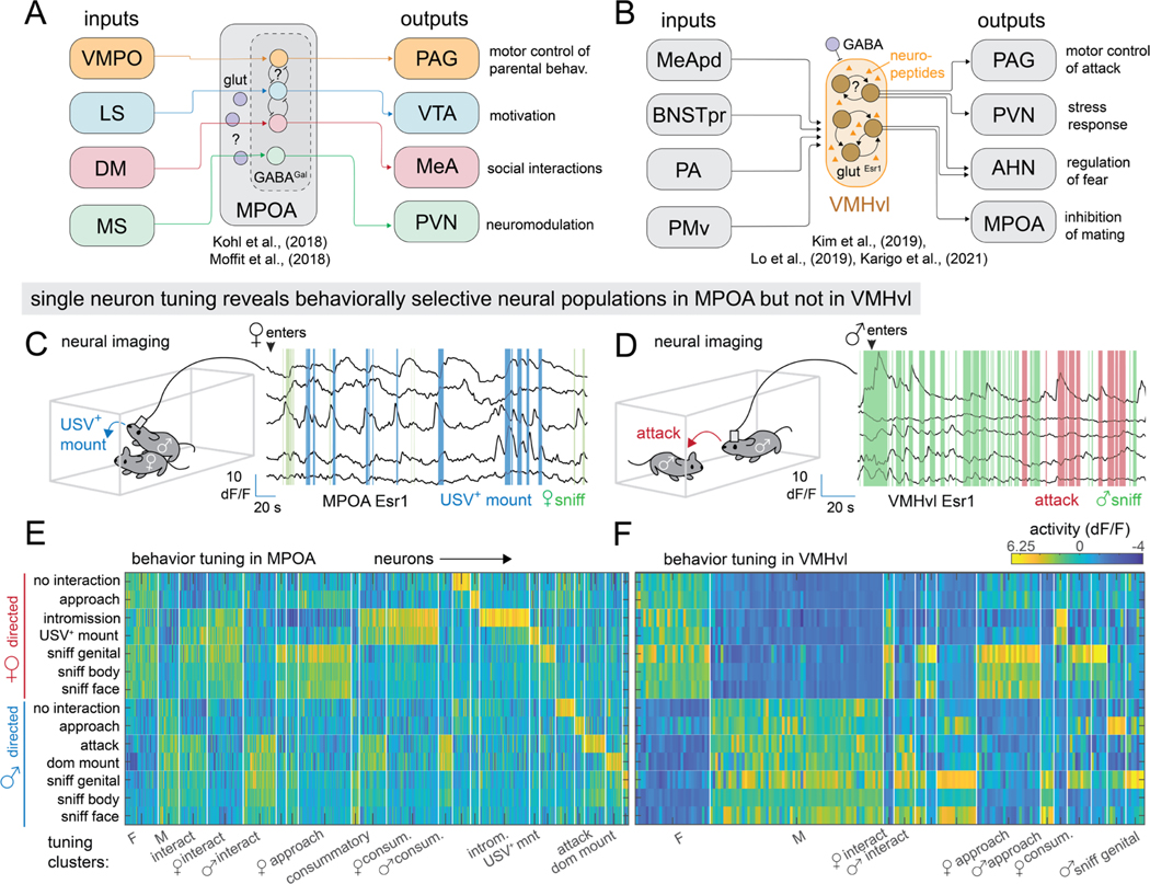
Figure 1:
Cytoarchitectures and cellular representations in a neural system regulating social behavior
A, B: cytoarchitecture of MPOA (A) and VMHvl (B). C, D: example traces from Esr1 + neurons in MPOA (C) and VMHvl (D). E, F: clustering of recorded Esr1 + neurons in MPOA (E, n =306 neurons from 3 mice...
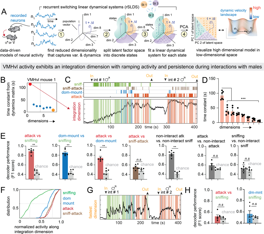
Figure 2:
Dynamical analysis of VMHvl neural activity reveals an integrator dimension that correlates with aggressive escalation
A: schematic illustrating rSLDS analysis. B: time constants of rSLDS dimensions (see Au2780) in attack enriched state from VMHvl mouse 1. Dimensions with longest (red dot) and shortest (yellow dot) ti...
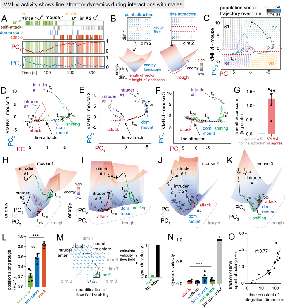
Figure 3:
VMHvl contains an approximate line attractor that integrates aggressive escalation
A: behavior rasters shown with first two principal components of dynamical system (see Methods ) for example VMHvl mouse 1. B: inferred dynamics shown as a flow field (with attractor highlighted) and ...
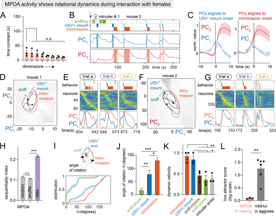
Figure 4:
Mating behaviors are represented using rotational dynamics in the MPOA
A: time constants of rSLDS dimensions in mating behavior-enriched state in MPOA (n = 3 mice) B: behavior rasters shown with first two principal components of latent factors for example MPOA mouse 2. C...
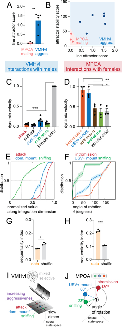
Figure 5:
Distinct neural coding schemes for similar behavior in VMHvl vs MPOA
A: line attractor score for mating behavior in MPOA and aggressive behavior in VMHvl (n = 3 mice for MPOA, n = 6 mice for VMHvl), reproduced from Figure 4L . B: scatter plot for line attractor score v...
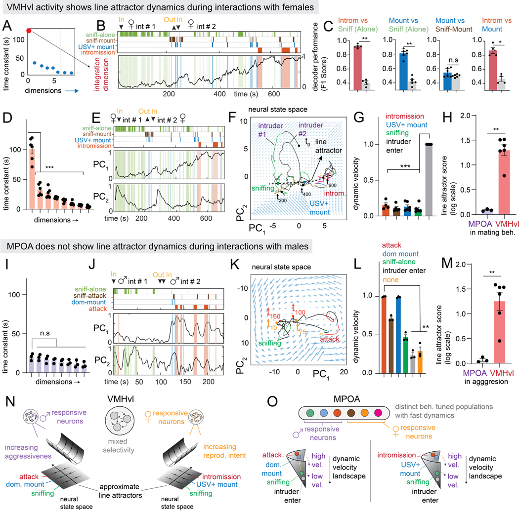
Figure 6:
Distinct coding schemes of VMHvl and MPOA are region-specific, not intruder-specific
A: left: time constants of rSLDS dimensions of mating enriched state from example VMHvl mouse 1. The red dot highlights the integration dimension. B: projection of integration dimension with overlayed...
Figure images are served from the NIH/NLM PubMed Central Open Access Subset or Europe PMC; copyright remains with the publishers and authors.
💬 Discussion
0 commentsNo comments yet. Be the first to start a discussion!
Leave a Comment