Abstract
Abstract Axonal structure underlies white matter functionality and plays a major role in brain connectivity. The current literature on the axonal structure is based on the analysis of two-dimensional (2D) cross-sections, which, as we demonstrate, is precarious. To be able to quantify three-dimensional (3D) axonal morphology, we developed a novel pipeline, called ACSON (AutomatiC 3D Segmentation and morphometry Of axoNs), for automated 3D segmentation and morphometric analysis of the white matter ultrastructure. The automated pipeline eliminates the need for time-consuming manual segmentation of 3D datasets. ACSON segments myelin, myelinated and unmyelinated axons, mitochondria, cells and vacuoles, and analyzes the morphology of myelinated axons. We applied the pipeline to serial block-face scanning electron microscopy images of the corpus callosum of sham-operated (n = 2) and brain injured (n = 3) rats 5 months after the injury. The 3D morphometry showed that cross-sections of myelinated axons were elliptic rather than circular, and their diameter varied substantially along their longitudinal axis. It also showed a significant reduction in the myelinated axon diameter of the ipsilateral corpus callosum of rats 5 months after brain injury, indicating ongoing axonal alterations even at this chronic time-point.
🔬 Techniques
💻 Software
✨ Fluorophores
🧪 Sample Preparation
🔬 Cell Lines
🏭 Microscope Brands
💻 Software Details
💾 Data Repositories
🏛️ Research Organizations (ROR)
Affiliated research institutions:
📋 Methods
Animal model, tissue preparation, and SBEM imaging Animals Five adult male Sprague-Dawley rats (10-weeks old, weight 320 and 380 g, Harlan Netherlands B.V., Horst, Netherlands) were used in the study. The animals were singly housed in a room (22 ± 1°C, 50–60% humidity) with 12 h light/dark cycle and free access to food and water. All animal procedures were approved by the Animal Care and Use Committee of the Provincial Government of Southern Finland and performed according to the guidelines set by the European Community Council Directive 86/609/EEC.
Traumatic brain injury model
TBI was induced by lateral fluid percussion injury in three rats (TBI-1, TBI-2, TBI-3) 62 . Rats were anesthetized with a single intraperitoneal injection (6 mL/kg) of a mixture of sodium pentobarbital (58 mg/kg), magnesium sulphate (127.2 mg/kg), propylene glycol (42.8%), and absolute ethanol (11.6%). A craniectomy (5 mm in diameter) was performed between bregma and lambda on the left convexity (anterior edge 2.0 mm posterior to bregma; lateral edge adjacent to the left lateral ridge). Lateral fluid percussion injury was induced in one rat by a transient fluid pulse impact (21 ms) against the exposed intact dura using a fluid-percussion device (Amscien Instruments, Richmond, VA, USA). The impact pressure was adjusted to 3.1 atm to induce a severe injury. Two sham-operated rats (Sham-1, Sham-2) underwent all the same surgical procedures except for the impact.
Tissue processing
Five months after TBI or sham operation, the rats were transcardially perfused using 0.9% NaCl (30 mL/min) for 2 min followed by 4% paraformaldehyde (30 mL/min) at 4 °C for 25 min. The brains were removed from the skull and post-fixed in 4% paraformaldehyde /1% glutaraldehyde overnight at 4 °C.
Show full methods section
Animal model, tissue preparation, and SBEM imaging Animals Five adult male Sprague-Dawley rats (10-weeks old, weight 320 and 380 g, Harlan Netherlands B.V., Horst, Netherlands) were used in the study. The animals were singly housed in a room (22 ± 1°C, 50–60% humidity) with 12 h light/dark cycle and free access to food and water. All animal procedures were approved by the Animal Care and Use Committee of the Provincial Government of Southern Finland and performed according to the guidelines set by the European Community Council Directive 86/609/EEC.
Traumatic brain injury model
TBI was induced by lateral fluid percussion injury in three rats (TBI-1, TBI-2, TBI-3) 62 . Rats were anesthetized with a single intraperitoneal injection (6 mL/kg) of a mixture of sodium pentobarbital (58 mg/kg), magnesium sulphate (127.2 mg/kg), propylene glycol (42.8%), and absolute ethanol (11.6%). A craniectomy (5 mm in diameter) was performed between bregma and lambda on the left convexity (anterior edge 2.0 mm posterior to bregma; lateral edge adjacent to the left lateral ridge). Lateral fluid percussion injury was induced in one rat by a transient fluid pulse impact (21 ms) against the exposed intact dura using a fluid-percussion device (Amscien Instruments, Richmond, VA, USA). The impact pressure was adjusted to 3.1 atm to induce a severe injury. Two sham-operated rats (Sham-1, Sham-2) underwent all the same surgical procedures except for the impact.
Tissue processing
Five months after TBI or sham operation, the rats were transcardially perfused using 0.9% NaCl (30 mL/min) for 2 min followed by 4% paraformaldehyde (30 mL/min) at 4 °C for 25 min. The brains were removed from the skull and post-fixed in 4% paraformaldehyde /1% glutaraldehyde overnight at 4 °C.
Tissue preparation for SBEM
The brains were sectioned into 1-mm thick coronal sections with a vibrating blade microtome (VT1000s, Leica Instruments, Germany). From each brain, a section at approximately 3.80 mm from bregma was selected and two samples from the ipsilateral and the contralateral corpus callosum were further dissected, as shown in Supplementary Fig. S6a . The samples were stained using an enhanced staining protocol 63 (see Supplementary Fig. S6b ). First, the samples were immersed in 2% paraformaldehyde in 0.15 M cacodylate buffer containing 2 mM calcium chloride (pH = 7.4), and then washed five times for 3 min in cold 0.15 Μ cacodylate buffer containing 2 mM calcium chloride (pH = 7.4). After washing, the samples were incubated for 1 h on ice in a solution containing 3% potassium ferrocyanide in 0.3 M cacodylate buffer with 4 mM calcium chloride combined with an equal volume of 4% aqueous osmium tetroxide. They were then washed in double distilled H2O (ddH2O) at room temperature (5 × 3 min). Thereafter, the samples were placed in a solution of 0.01 mg/mL thiocarbohydrazide solution at room temperature for 20 min. The samples were then rinsed again in ddH2O (5 × 3 min), and placed in 2% osmium tetroxide in ddH2O at room temperature. Following the second exposure to osmium, the samples were washed in ddH2O (5 × 3 min), and then incubated in 1% uranyl acetate overnight at 4 °C. The following day, the samples were washed in ddH2O (5 × 3 min) and en bloc Walton’s lead aspartate staining was performed. In this step, the samples were incubated in 0.0066 mg/mL lead nitrate in 0.03 M aspartic acid (pH = 5.5) at 60 °C for 30 min, after which the samples were washed in ddH2O at room temperature (5 × 3 min), and dehydrated using ice-cold solutions of freshly prepared 20%, 50%, 70%, 90%, 100%, and 100% (anhydrous) ethanol for 5 min each, and finally placed in ice-cold anhydrous acetone at room temperature for 10 min. Embedding was performed in Durcupan ACM resin (Electron Microscopy Sciences, Hatfield, PA, USA). First, the samples were placed into 25% Durcupan #1 (without component C):acetone, then into 50% Durcupan #1 :acetone, and after into 75% Durcupan #1 :acetone overnight. The following day, they were placed in 100% Durcupan #1 for 2 in a 50 oven (2 times), and into 100% Durcupan #2 (4-component mixture) for 2 h in a 50 °C oven. Finally, the samples were embedded in 100% Durcupan #2 in Beem embedding capsules (Electron Microscopy Sciences) and baked in a 60 °C oven for 48 h. After selecting the area within the samples, as shown in Supplementary Fig. S6c , the blocks were further trimmed into a pyramidal shape with a 1 × 1 mm 2 base and an approximately 600 × 600 μm 2 top (face), which assured the stability of the block while being cut in the SBEM microscope. The tissue was exposed on all four sides, bottom, and top of the pyramid. The blocks were then mounted on aluminum specimen pins using conductive silver epoxy (CircuitWorks CW2400). Silver paint (Ted Pella, Redding, CA, USA) was used to electrically ground the exposed block edges to the aluminum pins, except for the block face or the edges of the embedded tissue. The entire surface of the specimen was then sputtered with a thin layer of platinum coating to improve conductivity and reduce charging during the sectioning process. SBEM data acquisition All SBEM data were acquired on an SEM microscope (Quanta 250 Field Emission Gun; FEI Co., Hillsboro, OR, USA), equipped with the 3View system (Gatan Inc., Pleasanton, CA, USA) using a backscattered electron detector (Gatan Inc.). The top of the mounted block or face was the x-y plane, and the z direction was the direction of the cutting. All the samples were imaged with a beam voltage of 2.5 kV and a pressure of 0.15 Torr. The datasets were acquired with a resolution of 13-18.3 nm × 13-18.3 nm × 50 nm amounting to an area of 13.3-18.7 μm × 13.3-18.7 μm × 14.25 μm in the x , y , and z directions, respectively. After imaging, Microscopy Image Browser 14 was used to apply lateral registration to the slices. We quantified the registration using cross correlation analysis between successive slices and subtracting the running average (window size = 25) to preserve the directionality of axons while registration. Supplementary Fig. S6d shows a representative SBEM volume of the contralateral corpus callosum of the sham-operated rat. We also show two representative images cropped from the sham-operated and TBI volumes in Supplementary Fig. S6e and f, respectively. ACSON segmentation pipeline The ACSON segmentation pipeline annotates the ultrastructure in SBEM volumes of white matter. The pipeline began with denoising of the SBEM volumes, and proceeded by segmenting the volumes using BVG. The segmented volumes were refined using supervoxel techniques, and, finally, the subcellular structures, cells, and myelinated and unmyelinated axons were annotated.
Denoising
SBEM images are degraded by noise from different sources, such as noise in the primary beam, secondary emission noise, and noise in the final detection system 64 . To suppress these complex noise patterns, we applied a non-local BM4D algorithm 65 . Unlike local averaging filters, which smooth an image by averaging values in the neighborhood of a target voxel, non-local filtering considers all the voxels in the image, weighted by how similar these voxels are to the target voxel. BM4D, in particular, enhances a sparse representation in the transform-domain by grouping similar 3D image patches (i.e., continuous 3D blocks of voxels) into 4D data arrays called, groups. The steps to realize the filtering are the 4D transformation of 4D groups, shrinkage of the transform spectrum, and inverse 4D transformation. While BM4D has been extensively used for denoising datasets from diverse imaging modalities, its application in 3D-SBEM datasets is novel. We applied the default parameter values of BM4D for denoising, which automatically estimates the noise type and variance. Figure 1a shows a slice of SBEM volume before filtering, and Fig. 1b illustrates the BM4D output in which the noise has been strongly attenuated.
Segmentation
For the segmentation of a 3D-SBEM image, we devised a hybrid technique, named BVG, that integrates seeded region growing and edge detection. To elaborate BVG, we denote a 3D-SBEM image after denoising with BM4D as z ( x ): X → [0, 1], where x ∈ X is a 3D spatial coordinate. Note that the intensity can range from 0 to 1. We defined documentclass[12pt]{minimal} usepackage{amsmath} usepackage{wasysym} usepackage{amsfonts} usepackage{amssymb} usepackage{amsbsy} usepackage{mathrsfs} usepackage{upgreek} setlength{oddsidemargin}{-69pt} begin{document}$$hat{E}subset X$$end{document} E ˆ ⊂ X as the set of edges of z , using a Canny edge detector 66 . We set the parameter values of the Canny edge detector as follows: the SD of the Gaussian filter was documentclass[12pt]{minimal} usepackage{amsmath} usepackage{wasysym} usepackage{amsfonts} usepackage{amssymb} usepackage{amsbsy} usepackage{mathrsfs} usepackage{upgreek} setlength{oddsidemargin}{-69pt} begin{document}$$,sqrt{2}$$end{document} 2 and thresholds for weak and strong edges were 0.25 and 0.6 times the maximum gradient magnitude. In SBEM volumes with resolution anisotropy and a coarser resolution in the z direction, regions in successive slices did not appear continuously, and areas close to the structure boundaries overlapped. Therefore, we dilated the set of edge coordinates documentclass[12pt]{minimal} usepackage{amsmath} usepackage{wasysym} usepackage{amsfonts} usepackage{amssymb} usepackage{amsbsy} usepackage{mathrsfs} usepackage{upgreek} setlength{oddsidemargin}{-69pt} begin{document}$$hat{E}$$end{document} E ˆ in-plane with a 3 × 3 square structuring element. The dilated edges are denoted as E . The edge dilation was proportional to the resolution anisotropy. We then used BVG to segment z into n + 1 distinct volumes V 1 , V 2 , …, V n , E ⊂ X , in which V i ∩ V j = documentclass[12pt]{minimal} usepackage{amsmath} usepackage{wasysym} usepackage{amsfonts} usepackage{amssymb} usepackage{amsbsy} usepackage{mathrsfs} usepackage{upgreek} setlength{oddsidemargin}{-69pt} begin{document}$$varnothing $$end{document} ∅ , V i ∩ E = documentclass[12pt]{minimal} usepackage{amsmath} usepackage{wasysym} usepackage{amsfonts} usepackage{amssymb} usepackage{amsbsy} usepackage{mathrsfs} usepackage{upgreek} setlength{oddsidemargin}{-69pt} begin{document}$$varnothing $$end{document} ∅ , ∀ i , j = 1, …, n , i ≠ j . BVG is a serial segmentation algorithm, meaning that segmentation of V i starts only when V i −1 is segmented. To segment V i , BVG begins with one voxel called the seed, denoted as S k ⊂ V i , which iteratively grows— k is the iteration number—and finally results in the volume V i . N ( S k ) is in the neighborhood of S k defined as N ( S k ) = { r | r ∉ S k , ∃ s ∈ S k : r ∈ N ( s ), r ∉ E , r ∉ V 1,…, i −1 }, where N ( s ) is the 3D-neighborhood of voxel s . In each iteration, BVG appends a set of voxels A to S k , where A = { x | x ∈ N ( S k ), δ ( x ) ≤ δ T } and δ ( x ) measures the similarity of voxel x to the set S k . We defined the measure of similarity as documentclass[12pt]{minimal} usepackage{amsmath} usepackage{wasysym} usepackage{amsfonts} usepackage{amssymb} usepackage{amsbsy} usepackage{mathrsfs} usepackage{upgreek} setlength{oddsidemargin}{-69pt} begin{document}$$delta (x)=|z(x)-frac{1}{|{S}_{k}|}sum _{sin {S}_{k}}z(s)|$$end{document} δ ( x ) = | z ( x ) − 1 | S k | ∑ s ∈ S k z ( s ) | and set the similarity threshold δ T to 0.1. An iteration terminates, if A = documentclass[12pt]{minimal} usepackage{amsmath} usepackage{wasysym} usepackage{amsfonts} usepackage{amssymb} usepackage{amsbsy} usepackage{mathrsfs} usepackage{upgreek} setlength{oddsidemargin}{-69pt} begin{document}$$varnothing $$end{document} ∅ , or | S k | ≥ ϑ , where ϑ is a volume constraint. If V i grew larger than ϑ , the results were discarded and the voxels within V i were freed for other regions to compete for them. The segmentation was initiated by annotating the low-intensity structures, i.e., myelin and mitochondria, which were considered together as V 1 . BVG was initiated with a random low-intensity voxel S 1 with z ( S 1 ) ≤ 0.4. This one seed was sufficient to segment V 1 because myelin is a connected structure in a consecutive SBEM image. We defined N ( s ) using 26 neighbors, and set ϑ = ∞. Figure 1c shows a slice of canny edges together with the segmented myelin and mitochondria ( V 1 ). To segment other structures V 2 , …, V n , we needed a more advanced seeding mechanism. Referring to Fig. 1c , we noticed that other structures are surrounded by myelin and edges. Therefore, we first generated a binary mask, B , of the union of the dilated edges E and the myelin-mitochondria segment V 1 (Fig. 1c ). Denoting each 2D-slice of B as B i , we computed the Euclidean distance transform 67 for every B i individually, defined as DT i and shown in Fig. 1d . The pixel value in the distance transform DT i is the shortest distance from that pixel to a set of pixels B i . We defined the location of the seeds by extracting the regional maxima of each DT i (Fig. 1d ). To segment V i , BVG was initiated with a seed from the set of extracted regional maxima not belonging to any previously segmented V j , j = 1, …, i − 1. We defined N ( s ) using 6 neighbors and set ϑ = 10 6 , which equals 12.5 μm 3 of tissue or 1.5 times the volume of the largest axons in the dataset. Figure 1e shows one slice of the primary segmentation of the white matter ultrastructure, not belonging to B . The seed extraction overestimates the number of segmented volumes. This does not pose a problem, however, as the serial nature of BVG does not permit repetitive segmentation of an already segmented volume.
Segmentation post processing
The segmentation with BVG may result in small volumes, e.g., smaller than 5 × 10 3 voxels, which actually belong to larger segments. As well, dilated Canny edges E should be assigned with a label as Fig. 1f shows. Therefore, we refined the segmentation by utilizing the SLIC supervoxel 68 technique to relabel the small volumes and attach them to larger ones. Supervoxels group nearby voxels with similar intensity values into clusters. Particularly, SLIC clusters voxels based on a distance measure defined by documentclass[12pt]{minimal} usepackage{amsmath} usepackage{wasysym} usepackage{amsfonts} usepackage{amssymb} usepackage{amsbsy} usepackage{mathrsfs} usepackage{upgreek} setlength{oddsidemargin}{-69pt} begin{document}$${D}_{s}={d}_{int}+frac{c}{rho }{d}_{sp}$$end{document} D s = d i n t + c ρ d s p , where d int ensures intensity similarity and d sp enforces voxel proximity to the supervoxels. In SLIC, the initial supervoxel centers are defined at regular grid steps ρ , and their compactness is controlled by c . Also, the spacing parameter s allows accounting for resolution anisotropy in x , y , and z directions. We assigned the SLIC arguments to produce compact and large supervoxels, while accounting for the resolution anisotropy. Thus, we set c = 23, ρ = 11 and s = [1, 1, vx / vz ], where vx and vz are the voxel size in x and z directions, respectively. Note that, voxel size in x and y directions was equal. Supplementary Fig. S7 shows the effect of altering ρ , c and s while generating supervoxels. We refined the large volumes V i with more than 5 × 10 3 voxels by the SLIC supervoxels. In more detail, suppose that we have generated Q supervoxels SV q , q = 1, …, Q . Then, we re-defined V i as documentclass[12pt]{minimal} usepackage{amsmath} usepackage{wasysym} usepackage{amsfonts} usepackage{amssymb} usepackage{amsbsy} usepackage{mathrsfs} usepackage{upgreek} setlength{oddsidemargin}{-69pt} begin{document}$${V}_{i}^{^{prime} }=mathop{cup }limits_{qin I}S{V}_{q}$$end{document} V i ′ = ∪ q ∈ I S V q where documentclass[12pt]{minimal} usepackage{amsmath} usepackage{wasysym} usepackage{amsfonts} usepackage{amssymb} usepackage{amsbsy} usepackage{mathrsfs} usepackage{upgreek} setlength{oddsidemargin}{-69pt} begin{document}$$I={q^{prime} |frac{|S{V}_{q^{prime} }cap {V}_{i}|}{|S{V}_{q^{prime} }|}ge mathrm{0.8,}forall j < i:frac{|S{V}_{q^{prime} }cap {V}_{j}|}{|S{V}_{q^{prime} }|}mathrm{ < 0.8}}$$end{document} I = { q ′ | | S V q ′ ∩ V i | | S V q ′ | ≥ 0.8, ∀ j < i : | S V q ′ ∩ V j | | S V q ′ | 10}}^{4}$$end{document} | V i ′ |>10 4 , using a 3D distance transform, we propagated the surface of the volume for 1 μm. The surface of the enlarged volume was then propagated for −1 μm shrinking of the volume. Applying this procedure to each large volume altered the morphology of the volume, and closed those cavities smaller than 1 μm. The difference between the altered volume and V ′ was considered a potential mitochondrion, M i . We refined M i with SLIC supervoxels with the same parameter values and techniques mentioned in the segmentation post-processing section. Note that because some of the cavities were due to myelin, annotating the mitochondria was finalized using human supervision to check for myelin. Figure 1g shows the final result of the mitochondria segmentation. The myelin segment was then re-defined as the set difference of V 1 and all mitochondria, denoted as MY . In our SBEM-datasets, vacuoles appeared brighter than all of the other ultrastructures. Thus, if documentclass[12pt]{minimal} usepackage{amsmath} usepackage{wasysym} usepackage{amsfonts} usepackage{amssymb} usepackage{amsbsy} usepackage{mathrsfs} usepackage{upgreek} setlength{oddsidemargin}{-69pt} begin{document}$$|{V}_{i}^{^{prime} }| < 2times {10}^{4}$$end{document} | V i ′ | < 2 × 10 4 and documentclass[12pt]{minimal} usepackage{amsmath} usepackage{wasysym} usepackage{amsfonts} usepackage{amssymb} usepackage{amsbsy} usepackage{mathrsfs} usepackage{upgreek} setlength{oddsidemargin}{-69pt} begin{document}$$frac{1}{|{V}_{i}^{^{prime} }|}sum _{forall sin {V}_{i}^{text{'}}}z(s)ge 0.85$$end{document} 1 | V i ′ | ∑ ∀ s ∈ V i ' z ( s ) ≥ 0.85 , we labeled documentclass[12pt]{minimal} usepackage{amsmath} usepackage{wasysym} usepackage{amsfonts} usepackage{amssymb} usepackage{amsbsy} usepackage{mathrsfs} usepackage{upgreek} setlength{oddsidemargin}{-69pt} begin{document}$${V}_{i}^{^{prime} }$$end{document} V i ′ as a vacuole. We defined the remaining volumes, not mitochondria nor vacuole, as axons denoted as AX i , i = 1, …, m . To distinguish if an axon AX i was a myelinated or an unmyelinated axon, we studied a thick hollow cylinder enclosing the axon. The enclosing cylinder was formed by those supervoxels having a common face with the axon AX i . If the enclosing cylinder contained myelin above a threshold, the axon has been considered as a myelinated axon. In more detail, let Λ i be the indexes of supervoxels enclosing an axon AX i . If documentclass[12pt]{minimal} usepackage{amsmath} usepackage{wasysym} usepackage{amsfonts} usepackage{amssymb} usepackage{amsbsy} usepackage{mathrsfs} usepackage{upgreek} setlength{oddsidemargin}{-69pt} begin{document}$$frac{|(mathop{cup }limits_{qin {{rm{Lambda }}}_{i}}S{V}_{q}),cap MY|}{|{(mathop{cup }limits_{qin {{rm{Lambda }}}_{i}}SV)}_{q}|}ge 0.7$$end{document} | ( ∪ q ∈ Λ i S V q ) ∩ M Y | | ( ∪ q ∈ Λ i S V ) q | ≥ 0.7 , we considered AX i to be a myelinated axon. Note that because unmyelinated axons can be surrounded by several myelinated axons, they can be miss-classified as myelinated axons, thus requiring a proof reading after the classification. To label cells and cell-processes, we considered a straightforward approach as the volumes of cells were expected to be larger than the volumes of any other structure, excluding myelin. Recall that we set the volume threshold ϑ = 10 6 for the segmentation of V 2 , …, V n , which leaves some voxels unlabeled. These unlabeled voxels X ′ comprised cells and cell processes. We segmented X ′ into n ′ cells using connected component analysis. In general, we detected 1–4 cell bodies/process in each SBEM-volume. Figure 1h demonstrates the final segmentation results of myelin, myelinated axons, unmyelinated axons, oligodendrocyte cell body and its processes. Mitochondria and vacuoles belonging to myelinated axons were colored the same as their corresponding myelinated axons. Figure 1i and Supplementary Fig. S4 show the 3D rendering of myelinated axons in contralateral corpus callosum of Sham-1 dataset.
ACSON morphometry pipeline
We defined a cross-section as the intersection of a segmented myelinated axon Ω and a perpendicular plane to the axonal skeleton γ 69 . To detect the myelinated axon skeleton γ with sub-voxel precision, we adapted a method from Van Uitert & Bitter 70 . First, we defined three points in the myelinated axon domain Ω: x * with the largest distance from the myelinated axon surface Γ, and x e 1 and x e 2 as the endpoints of the axons, i.e., the tips of the axon. The minimum-cost path connecting x e 1 to x e 2 through x * was the axon skeleton γ . The path was found in two steps, first from x e 1 to x *, and then from x e 2 to x *. Mathematically, 1 documentclass[12pt]{minimal} usepackage{amsmath} usepackage{wasysym} usepackage{amsfonts} usepackage{amssymb} usepackage{amsbsy} usepackage{mathrsfs} usepackage{upgreek} setlength{oddsidemargin}{-69pt} begin{document}$$gamma ={rm{arg }}mathop{{rm{min }}}limits_{P}{int }_{{x}_{e1}}^{{x}_{e2}}H(P(varsigma ))dvarsigma ,$$end{document} γ = arg min P ∫ x e 1 x e 2 H ( P ( ς ) ) d ς , where ς traces the path P , and H is the cost function. To enforce the minimum-cost path to run at the middle of the object, the cost function H should be higher if the path moves away from the center. Points x *, x e 1 , and x e 2 and solving equation ( 1 ) was defined by solving an eikonal equation on the axonal domain Ω. The eikonal equation is a non-linear partial differential equation defined as a special case of wave propagation in which the front Γ advances monotonically with speed F ( x ) > 0. The eikonal equation can be formulated as |∇ T ( x )| F ( x ) = 1, where T | Γ = 0. The solution, T ( x ), is the shortest time needed to travel from Γ to any point x ∈ Ω, with the speed F ( x ) > 0. Although the eikonal equation can be solved with the FMM 71 , we used 3D MSFM 51 . MSFM combines multiple stencils and second-order approximation of the directional derivatives over the FMM to improve the accuracy of solving the eikonal equation on Cartesian domains. To find x *, we computed the time-crossing map T 1 ( x ) from the myelinated axon interface Γ with constant speed F 1 ( x ) = 1, x ∈ Ω. The global maximum of T 1 , where T 1 ( x ) ≤ T 1 ( x *), ∀ x ∈ Ω was defined as x *. To find x e 1 , x e 2 , and γ , we calculated a new time-crossing map T 2 ( x ), starting at x * to every voxel in Ω, with a non-constant speed documentclass[12pt]{minimal} usepackage{amsmath} usepackage{wasysym} usepackage{amsfonts} usepackage{amssymb} usepackage{amsbsy} usepackage{mathrsfs} usepackage{upgreek} setlength{oddsidemargin}{-69pt} begin{document}$${F}_{2}(x)={(frac{{T}_{1}(x)}{{T}_{1}({x}^{ast })})}^{2}$$end{document} F 2 ( x ) = ( T 1 ( x ) T 1 ( x ⁎ ) ) 2 for x ∈ Ω. T 1 ( x )| Γ = 0. Using H ( x ) = 1 − F 2 ( x ) to define the cost ensured that voxels in the middle of the myelinated axon were reached prior to the voxels close to Γ. We defined the furthest point from x * on the T 2 map, i.e., the global maximum of T 2 , as x e 1 . Similarly, x e 2 was defined as the furthest point from x e 1 , at the global maximum of the time-crossing map T 3 ( x ), starting from x e 1 to every voxel in Ω, with speed F 2 ( x ). For both endpoints, we determined the minimum-cost path between x ei and x *, γ i , i = 1, 2, by backtracking, starting from x ei and progressing along the negative gradient documentclass[12pt]{minimal} usepackage{amsmath} usepackage{wasysym} usepackage{amsfonts} usepackage{amssymb} usepackage{amsbsy} usepackage{mathrsfs} usepackage{upgreek} setlength{oddsidemargin}{-69pt} begin{document}$$-frac{nabla {T}_{2}(x)}{|nabla {T}_{2}(x)|}$$end{document} − ∇ T 2 ( x ) | ∇ T 2 ( x ) | until x * was reached. x * is the global minimum of T 2 ( x ), so that we were guaranteed to find it with backtracking. The backtracking procedure can be described by the ordinary differential equation documentclass[12pt]{minimal} usepackage{amsmath} usepackage{wasysym} usepackage{amsfonts} usepackage{amssymb} usepackage{amsbsy} usepackage{mathrsfs} usepackage{upgreek} setlength{oddsidemargin}{-69pt} begin{document}$$frac{d{gamma }_{i}}{dvarsigma }=-frac{nabla {T}_{2}}{|nabla {T}_{2}|},,{gamma }_{i}(varsigma =0)mathrm{=}{x}_{ei}$$end{document} d γ i d ς = − ∇ T 2 | ∇ T 2 | , γ i ( ς = 0 ) = x e i , where ς traces γ i . We used a 4th order Runge-Kutta scheme, with a 25 nm step size, to solve the ordinary differential equation with sub-voxel accuracy. The myelinated axon skeleton was formed as γ = γ 1 ∪ γ 2 . Note that computing the skeleton in this way prevented the skeleton from cutting corners 72 . Figure 3a shows a 3D reconstruction of a myelinated axon, its mitochondria, and the extracted skeleton (axonal axis). Note that x e 1 and x e 2 defined as the global maxima of T 2 ( x ) and T 3 ( x ), lie on the myelinated axon surface Γ, and not in the center of the myelinated axon. The cost function H , however, forces the skeleton to immediately move away from the surface Γ toward the center. Therefore, we dropped the first 1 μm at both ends of γ in our later calculations. To determine the cross-sectional planes perpendicular to γ , we formed a moving reference frame of the size 8 μm × 8 μm with 50 nm resolution. At each skeleton point ς , the unit tangent vector to γ was used to define the orientation of the reference frame. The intersection of the reference frame with the myelinated axon defined the cross-section of the myelinated axon. The intensity values of a cross-section ranged between 0 and 1. Each cross-section was thresholded at 0.5, resulting in a 2D binary image C denoted as C : X → {0, 1}, where the point x = ( x 1 , x 2 ) was foreground iff x ∈ C . We defined the center point of C as documentclass[12pt]{minimal} usepackage{amsmath} usepackage{wasysym} usepackage{amsfonts} usepackage{amssymb} usepackage{amsbsy} usepackage{mathrsfs} usepackage{upgreek} setlength{oddsidemargin}{-69pt} begin{document}$$c=frac{1}{|C|}sum _{xin C}x$$end{document} c = 1 | C | ∑ x ∈ C x . By translating the binary 2D cross-section C to the center of 2D Cartesian coordinate C t = { y ∈ X : y = x − c }, we found an ellipse that had the same normalized second central moment as C t . The cross-sectional morphology of myelinated axons were quantified by computing the minor and major axes and the eccentricity of the fitted ellipse 73 , and the diameter of a circle with the same area as the cross-section, called equivalent diameter.
Evaluation of segmentation accuracy Manual segmentation
The manual segmentation by A.S. defined each ultrastructure as its own region, i.e., different axons had distinct labels in the manual segmentation as in the automatic one. It also annotated each segmented region as myelin, myelinated or unmyelinated axon. In the annotated images, mitochondria and vacuoles were included into intra-axonal space. Precision and recall For a tissue-type level evaluation, we used the precision and recall as in the previous studies 28 , 32 . Let A and B be the sets of voxels of a particular tissue-type (myelin, myelinated axon, unmyelinated axon) in the manual and automated segmentations, respectively. We defined documentclass[12pt]{minimal} usepackage{amsmath} usepackage{wasysym} usepackage{amsfonts} usepackage{amssymb} usepackage{amsbsy} usepackage{mathrsfs} usepackage{upgreek} setlength{oddsidemargin}{-69pt} begin{document}$$Precision=frac{|Acap B|}{|B|}$$end{document} P r e c i s i o n = | A ∩ B | | B | , and documentclass[12pt]{minimal} usepackage{amsmath} usepackage{wasysym} usepackage{amsfonts} usepackage{amssymb} usepackage{amsbsy} usepackage{mathrsfs} usepackage{upgreek} setlength{oddsidemargin}{-69pt} begin{document}$$Recall=frac{|Acap B|}{|A|}$$end{document} R e c a l l = | A ∩ B | | A | . The maximum for the precision and recall is equal to one when the automated segmentation perfectly matches the manual segmentation. These metrics do not describe topological differences between the manual and automated segmentations. For example, these metrics do not penalize the automatic segmentation for incorrectly dividing a single axon into two axons. Weighted Jaccard index and weighted Dice coefficient To further evaluate the automated segmentation, we used Jaccard index and Dice coefficients in the region level. The Jaccard index 74 and Dice coefficient 75 is defined by documentclass[12pt]{minimal} usepackage{amsmath} usepackage{wasysym} usepackage{amsfonts} usepackage{amssymb} usepackage{amsbsy} usepackage{mathrsfs} usepackage{upgreek} setlength{oddsidemargin}{-69pt} begin{document}$$J(A,B)=frac{|Acap B|}{|Acup B|}$$end{document} J ( A , B ) = | A ∩ B | | A ∪ B | and documentclass[12pt]{minimal} usepackage{amsmath} usepackage{wasysym} usepackage{amsfonts} usepackage{amssymb} usepackage{amsbsy} usepackage{mathrsfs} usepackage{upgreek} setlength{oddsidemargin}{-69pt} begin{document}$$Dice,Coef(A,B)=frac{mathrm{2|}Acap B|}{|A|+|B|}$$end{document} D i c e C o e f ( A , B ) = 2| A ∩ B | | A | + | B | , where A and B are the regions segmented manually and automatically, respectively. The maximum for these metrics is equal to one occurring when A perfectly matches B . If no overlap occurs between A and B , these metrics are equal to zero. Let A i , i = 1, …, a ′, and B j , j = 1, …, b ′ be the regions in the manual and automated segmentation, respectively. To assign A i and the best matching B j , we formed a similarity matrix based on Dice coefficients for any possible pair of A i and B j , where the element ( i , j ) of the similarity matrix was Dice Coef ( A i , B j ). We used the Hungarian algorithm 76 , 77 to match the regions. We defined the weighted mean of the Jaccard index and the weighted mean of the Dice coefficients as documentclass[12pt]{minimal} usepackage{amsmath} usepackage{wasysym} usepackage{amsfonts} usepackage{amssymb} usepackage{amsbsy} usepackage{mathrsfs} usepackage{upgreek} setlength{oddsidemargin}{-69pt} begin{document}$$sum _{imathrm{=1}}^{a^{prime} }{w}_{i}J({A}_{i},{B}_{b(i)})$$end{document} ∑ i =1 a ′ w i J ( A i , B b ( i ) ) , and documentclass[12pt]{minimal} usepackage{amsmath} usepackage{wasysym} usepackage{amsfonts} usepackage{amssymb} usepackage{amsbsy} usepackage{mathrsfs} usepackage{upgreek} setlength{oddsidemargin}{-69pt} begin{document}$$sum _{imathrm{=1}}^{a^{prime} }{w}_{i}Dice,Coef({A}_{i},{B}_{b(i)})$$end{document} ∑ i =1 a ′ w i D i c e C o e f ( A i , B b ( i ) ) , respectively, where b ( i ) is the index of the region best matching A i and the weight documentclass[12pt]{minimal} usepackage{amsmath} usepackage{wasysym} usepackage{amsfonts} usepackage{amssymb} usepackage{amsbsy} usepackage{mathrsfs} usepackage{upgreek} setlength{oddsidemargin}{-69pt} begin{document}$${w}_{i}=frac{|{A}_{i}|}{|{sum }_{imathrm{=1}}^{a^{prime} }{A}_{i}|}$$end{document} w i = | A i | | ∑ i =1 a ′ A i | .
Comparison of 2D and 3D morphological analyses
To simulate 2D morphometry, we assumed that the myelinated axon morphometry is quantified on a single image of the 3D image stack. For each myelinated axon, we determined the best orientation of the image stack for the 2D quantifications by extracting the Euler angles of a fitted ellipsoid to the segmented myelinated axon. We randomly selected a single image in that orientation to present the myelinated axon. For example, if a myelinated axon was elongated parallel to the z -axis, we selected a random image parallel to the x − y plane. Each myelinated axon was quantified separately for its minor and major axes, equivalent diameter, and eccentricity. The relative difference between the 2D and 3D quantifications for each myelinated axon was defined as documentclass[12pt]{minimal} usepackage{amsmath} usepackage{wasysym} usepackage{amsfonts} usepackage{amssymb} usepackage{amsbsy} usepackage{mathrsfs} usepackage{upgreek} setlength{oddsidemargin}{-69pt} begin{document}$$relative,difference=frac{|{q}_{2D}-{q}_{3D}|}{{rm{max }}({q}_{2D},{q}_{3D})}$$end{document} r e l a t i v e d i f f e r e n c e = | q 2 D − q 3 D | max ( q 2 D , q 3 D ) , where q is the quantity of interest, i.e., minor and major axes, equivalent diameter, and the eccentricity, measured by the 2D or 3D procedures. Note that, for the 3D morphometry, median of the measurements along the axonal axis were quantified Fig. 4a .
Statistical analysis Nested ANOVA
Nested (hierarchical) ANOVA is a parametric hypothesis testing and an extension of 1-way ANOVA. A nested ANOVA is used when there is one measurement variable and more than one nominal variable, and the nominal variables are nested 35 . The nominal variables being nested means that each value of one nominal variable (the subgroups) is found in combination with only one value of the higher-level nominal variable (the groups). We considered lower-level variables (cross-section, axon, animal) as random effects variables and the top level (group, either sham or TBI) as a fixed effect variable. The null hypotheses were whether there existed significant variation in means among groups at each level. The analysis was performed using the anovan function of MATLAB R2017b, with type II sum of squares. Because, the design matrix of anovan grows quickly when the nesting levels increases, we measured the median of the cross-sectional quantities and assigned them to the lowest level of nested ANOVA. At the cross-sectional level, the distributions of equivalent diameter, minor and major axes and eccentricity were multimodal (Supplementary Fig. S5 ), thus median of cross-sections was preferred to mean. The analysis was performed separately for two hemispheres. Variance components Nested ANOVA partitions the variability of the measurements into different levels. The variance components describe what percentage of the total variance is attributable to each level 35 .
Supplementary information Supplementary Information
📊 Figures
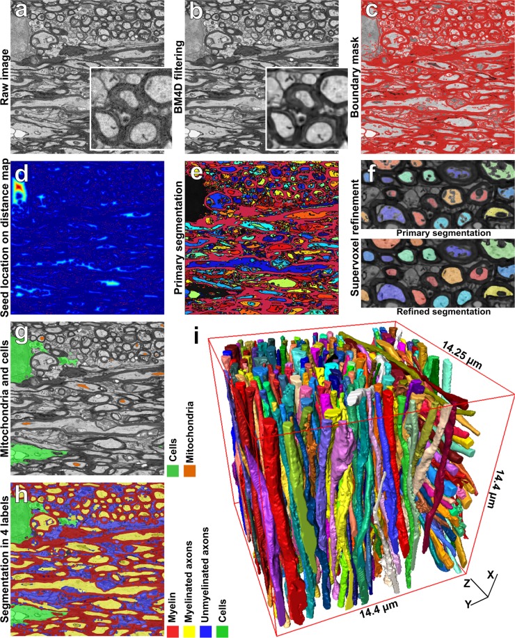
Figure 1
White matter ACSON segmentation pipeline. ( a ) A 2D representative image of the SBEM dataset from the contralateral corpus callosum of Sham-1 dataset. ( b ) The same image denoised with BM4D. ( c ) B...
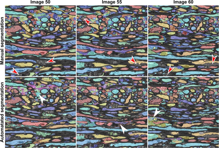
Figure 2
Manual expert segmentation and automated segmentation of three images from the contralateral corpus callosum of Sham-1 dataset. We used the Hungarian algorithm to match the color of segmented regions ...
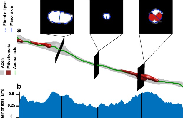
Figure 3
ACSON morphometry. ( a ) 3D reconstruction of a representative intra-axonal space of one myelinated axon and its mitochondria. Three intersecting planes at randomly selected positions show the cross-s...
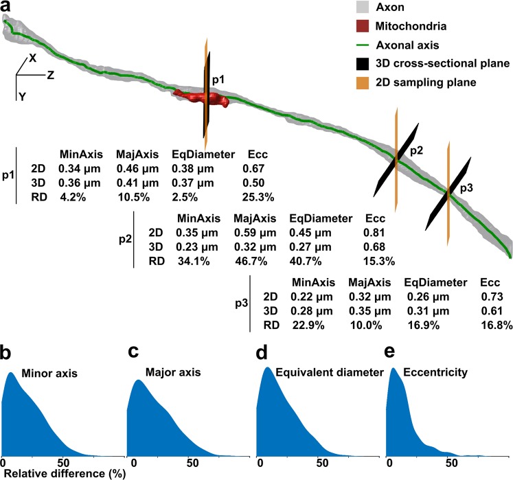
Figure 4
A comparison between the 2D and 3D morphological analyses. ( a ) 3D reconstruction of intra-axonal space of a representative myelinated axon with an axis that does not align with image cross-sections....
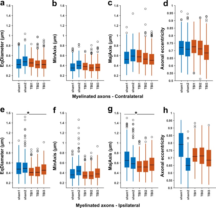
Figure 5
Box-plots of equivalent diameter (EqDiameter), minor axis (MinAxis), major axis (MajAxis), and axonal eccentricity measured for myelinated axons in sham-operated and TBI animals. The measurements are ...
Figure images are served from the NIH/NLM PubMed Central Open Access Subset or Europe PMC; copyright remains with the publishers and authors.
💬 Discussion
0 commentsNo comments yet. Be the first to start a discussion!
Leave a Comment