Abstract
Goal-directed behavior requires the interaction of multiple brain regions. How these regions and their interactions with brain-wide activity drive action selection is less understood. We have investigated this question by combining whole-brain volumetric calcium imaging using light-field microscopy and an operant-conditioning task in larval zebrafish. We find global, recurring dynamics of brain states to exhibit pre-motor bifurcations toward mutually exclusive decision outcomes. These dynamics arise from a distributed network displaying trial-by-trial functional connectivity changes, especially between cerebellum and habenula, which correlate with decision outcome. Within this network the cerebellum shows particularly strong and predictive pre-motor activity (>10 s before movement initiation), mainly within the granule cells. Turn directions are determined by the difference neuroactivity between the ipsilateral and contralateral hemispheres, while the rate of bi-hemispheric population ramping quantitatively predicts decision time on the trial-by-trial level. Our results highlight a cognitive role of the cerebellum and its importance in motor planning.
🔬 Techniques
🧬 Organisms
💻 Software
✨ Fluorophores
🧪 Sample Preparation
🏭 Microscope Brands
🔴 Lasers
📷 Detectors
💻 Software Details
💾 Data Repositories
🏛️ Research Organizations (ROR)
Affiliated research institutions:
📋 Methods
LEAD CONTACT AND MATERIALS AVAILABILITY
Further information and requests for resources should be directed to the lead contact, Alipasha Vaziri ( vaziri@rockefeller.edu ). This study did not generate new unique reagents.
EXPERIMENTAL MODEL AND SUBJECT DETAILS Animal Subjects
Experiments were carried out in accordance with protocols approved by the Institutional Animal Care and Use Committee. Zebrafish ( Danio rerio ) lines used in this study for imaging and behavioral experiments were 7–9 day-post-fertilization Tg(elavl3:H2B-GCaMP6s) ( Vladimirov et al., 2014 ) in Nacre or Casper mutant background. Adult fish were housed in a facility at 28.5 °C with lights on between 8 am and 10 pm. No statistical methods were used to pre-determine sample size. METHOD DETAILS Whole-brain Calcium Imaging with the Operant Conditioning Task, and Signal Extraction 7–9 day-post-fertilization zebrafish larvae were embedded in 2–2.5% low-melting-temperature agarose in a custom-made chamber on a glass slide and then immersed in fish water. The agarose around the tail, caudal to the swim bladder, was removed to free the tail of the larvae and then incubated for 6–8 hours for further solidification. Under this head-fixed condition, larvae were placed above a camera (Grasshopper3, PointGrey) for tracking tail movements at 160 Hz and placed under a 20×/0.5-NA water-immersion objective (Olympus) for whole-brain calcium imaging with an upright light-field microscope at 10 Hz ( Nöbauer et al., 2017 ; Prevedel et al., 2014 ). The tail was illuminated with a near-infrared (NIR) 950 nm light-emitting diode (LED), and GCaMP was excited with a blue LED (pe-2, CoolLED). Custom-written MATLAB (MathWorks) software was used to extract the tail angle, using the resting tail position as the reference, with positive angles representing right turns and zero degrees corresponding to a straight tail. Heat stimulus was delivered using 980-nm fiber-coupled laser (Roithner Lasertechnik), collimated via a collimator (Thorlabs, F220FC-1064) and then projected to the head of the fish along the midline, with the spot diameter of 2.0 mm (measured power: 300 mW). A 950-nm bandpass filter (FB950–10, Thorlabs) was placed in front of the Grasshopper camera to reject scattered visible light and crosstalk from the heat stimulus. Real-time heat stimuli were controlled by a data acquisition board (USB-6008, National Instruments) and modulated by the extracted tail angle exceeding a threshold (35°) in a closed loop. For movement events with multiple tail deflections, only the first deflection was considered. Image acquisition of the LFM was controlled using Micro-Manager ( Stuurman et al., 2007 ) and triggered by the custom MATLAB software. The whole setup was controlled from a dual-CPU workstation (Z820, HP). 3D reconstruction of the LFM images was carried out offline with the volume of ~700 μm × 700 μm × 200 μm with 51 z-planes and fed into a custom-written pipeline for neuronal signal extraction based on the approach proposed by ( Mukamel et al., 2009 ; Prevedel et al., 2014 ): The reconstructed LFM data, which is a timeseries of volumetric frames, was first de-trended by dividing each volumetric frame by a slowly-varying fit to the frame means. To reduce the data to an amount tractable by Independent Component Analysis (ICA), the variance over time was computed for each voxel, and the highest-variance voxels, as well as 2–3 continuous time ranges amounting to 10% of the total recording time were selected to serve as input data to the ICA. The entire recording volume was divided into 6 slightly overlapping sub-volumes. The selected voxels and timepoints were factorized independently for each sub-volume using the FastICA algorithm (initialized by PCA) ( Hyvärinen and Oja, 2000 ), resulting in a set of spatial filters and associated temporal signals. The spatial filters were thresholded to detect regions of interest (ROIs), and ROIs compatible with shape and size of neurons were kept. Duplicate ROIs in the overlapping sub-volume regions were merged, resulting in the final set of neuron spatial filters. Finally, the corresponding neuron activity signals were extracted from the original reconstructed LFM dataset by summing (for each timestep) over the voxel brightness values in each neuron spatial filter.
Show full methods section
LEAD CONTACT AND MATERIALS AVAILABILITY
Further information and requests for resources should be directed to the lead contact, Alipasha Vaziri ( vaziri@rockefeller.edu ). This study did not generate new unique reagents.
EXPERIMENTAL MODEL AND SUBJECT DETAILS Animal Subjects
Experiments were carried out in accordance with protocols approved by the Institutional Animal Care and Use Committee. Zebrafish ( Danio rerio ) lines used in this study for imaging and behavioral experiments were 7–9 day-post-fertilization Tg(elavl3:H2B-GCaMP6s) ( Vladimirov et al., 2014 ) in Nacre or Casper mutant background. Adult fish were housed in a facility at 28.5 °C with lights on between 8 am and 10 pm. No statistical methods were used to pre-determine sample size. METHOD DETAILS Whole-brain Calcium Imaging with the Operant Conditioning Task, and Signal Extraction 7–9 day-post-fertilization zebrafish larvae were embedded in 2–2.5% low-melting-temperature agarose in a custom-made chamber on a glass slide and then immersed in fish water. The agarose around the tail, caudal to the swim bladder, was removed to free the tail of the larvae and then incubated for 6–8 hours for further solidification. Under this head-fixed condition, larvae were placed above a camera (Grasshopper3, PointGrey) for tracking tail movements at 160 Hz and placed under a 20×/0.5-NA water-immersion objective (Olympus) for whole-brain calcium imaging with an upright light-field microscope at 10 Hz ( Nöbauer et al., 2017 ; Prevedel et al., 2014 ). The tail was illuminated with a near-infrared (NIR) 950 nm light-emitting diode (LED), and GCaMP was excited with a blue LED (pe-2, CoolLED). Custom-written MATLAB (MathWorks) software was used to extract the tail angle, using the resting tail position as the reference, with positive angles representing right turns and zero degrees corresponding to a straight tail. Heat stimulus was delivered using 980-nm fiber-coupled laser (Roithner Lasertechnik), collimated via a collimator (Thorlabs, F220FC-1064) and then projected to the head of the fish along the midline, with the spot diameter of 2.0 mm (measured power: 300 mW). A 950-nm bandpass filter (FB950–10, Thorlabs) was placed in front of the Grasshopper camera to reject scattered visible light and crosstalk from the heat stimulus. Real-time heat stimuli were controlled by a data acquisition board (USB-6008, National Instruments) and modulated by the extracted tail angle exceeding a threshold (35°) in a closed loop. For movement events with multiple tail deflections, only the first deflection was considered. Image acquisition of the LFM was controlled using Micro-Manager ( Stuurman et al., 2007 ) and triggered by the custom MATLAB software. The whole setup was controlled from a dual-CPU workstation (Z820, HP). 3D reconstruction of the LFM images was carried out offline with the volume of ~700 μm × 700 μm × 200 μm with 51 z-planes and fed into a custom-written pipeline for neuronal signal extraction based on the approach proposed by ( Mukamel et al., 2009 ; Prevedel et al., 2014 ): The reconstructed LFM data, which is a timeseries of volumetric frames, was first de-trended by dividing each volumetric frame by a slowly-varying fit to the frame means. To reduce the data to an amount tractable by Independent Component Analysis (ICA), the variance over time was computed for each voxel, and the highest-variance voxels, as well as 2–3 continuous time ranges amounting to 10% of the total recording time were selected to serve as input data to the ICA. The entire recording volume was divided into 6 slightly overlapping sub-volumes. The selected voxels and timepoints were factorized independently for each sub-volume using the FastICA algorithm (initialized by PCA) ( Hyvärinen and Oja, 2000 ), resulting in a set of spatial filters and associated temporal signals. The spatial filters were thresholded to detect regions of interest (ROIs), and ROIs compatible with shape and size of neurons were kept. Duplicate ROIs in the overlapping sub-volume regions were merged, resulting in the final set of neuron spatial filters. Finally, the corresponding neuron activity signals were extracted from the original reconstructed LFM dataset by summing (for each timestep) over the voxel brightness values in each neuron spatial filter.
Training Protocol and Animal Behavior
We aimed to find a robust behavioral paradigm that involved learning and short-term memory while exhibiting a delay period from the onset of an instructing sensory cue to the execution of motor response, during which the neuronal basis of motor planning and decision making could be studied. While previously used assays in larval zebrafish for sensorimotor transformation lack the above features, most of the typically used assays in rodents or primates study motor planning by introducing a delay period from the onset of the stimulus to a go cue, after which the animal is trained to initiate a motor response (Mohebi and Oweiss, 2014; Shenoy et al., 2013 ; Svoboda and Li, 2018 ). However, motor responses of animals engaged in naturalistic action selections are self-initiated and happen in the absence of a go cue. The ROAST operant conditioning paradigm ( Figure 1A ) addresses both issues. Typically, each recording consisted of 20–25 trials and lasted for one hour. In each trial, heat stimulus was delivered 5 seconds after the trial started and was terminated immediately when a turn in the correct direction exceeded a threshold (35 degree). If an animal failed to make a correct movement within 100 s, the laser was switched off and the fish received a 20 s break before the start of the next trial. Otherwise, if an animal made a correct movement, the heat stimulus was turned off and the fish received a break for the rest of the 100 s trial. The full training protocol for each fish consisted of two training blocks (one left- and one right-training block), with each block containing 20–25 trials. Since individual fish exhibited a bias for a specific direction ( Li, 2013 ), the reward direction in the first training block was chosen against this bias and was subsequently reversed in the second block. Prior to the first block, 3–5 probe trials were conducted to determine the pre-existing bias of individual fish. For “learners” (see below), the same larvae were imaged twice for two training blocks, over a total of two hours, and with a 0.5 h break in between. A given trial was classified as correct when the first heat-evoked turn of the animal was in the reward direction, and a fish was defined as a “learner” when the asymptote of the learning curve (modelled by a sigmoidal function that was fit to the outcomes) in both blocks reached a threshold of 70% correct. Fish that learned in the first but not in the second block were defined as intermediate learners and their data was not included in the data analysis. If a fish failed to learn in the first block, it was categorized as a non-learner and was not considered further for the second training block. Overall, we behaviorally trained and recorded data from 26 larvae resulting in 39% learners, 46% non-learners and 15% intermediate learners, which were not included in further analyses. In all further analyses, training blocks were analyzed separately, such that a “correct trial” always corresponded to a turn in the left or right direction. Pre-processing of the Neuronal Signals Each neuronal time series was de-trended individually to correct for photo-bleaching, and then normalized as ΔF/F0 = (F-F0)/F0, where F is the fluorescence of the neuron at a given timepoint and F0 is the average fluorescence of the neuron across the entire recording. Noise was removed via total variation regularization by calculating the cumulative sum of the de-noised time derivatives ( Chartrand, 2011 ). The de-noised time series X of each neuron were then normalized by taking the Z-score, given as (X – mean(X))/SD(X), for further analysis. This pre-processing procedure and subsequent analyses were performed using MATLAB (MathWorks).
Behavior Classification
In addition to online tracking, offline behavioral classification was used to classify the tail movements as left turns, right turns, and struggles (or swimming), using a method similar to the one described by ( Haesemeyer et al., 2018 ). Briefly, since larval zebrafish move in bouts rather than swim continuously, and since the bout duration lasts for about 250–400 ms in head-restrained fish ( Severi et al., 2014 ), the movement bout was detected by scanning through the time series of the tracked tail angle in a sliding window of 50 frames (corresponding to ~312 ms at a frame rate of 160 Hz). Within the time window of one bout, the time of movement initiation was set to the timepoint when the tail angle exceeded 5° for the first time. Then, the bias of tail movements was calculated, and the bout was categorized as a unilateral ‘turn’ or a bilateral ‘struggle’ with the threshold of bias at 1.05. The turn direction was determined from the sign of the tail angle, negative or positive, for left and right turns (labelled “TurnL” and “TurnR”), respectively. Decision Time Decision time (DT) was measured as the time between heat onset to the initiation of the first turn, regardless of correct or incorrect outcome, in a given trial. Because the temperature changes from the heat stimulus became relatively stable 5 s after heat onset, only trials with DT longer than 5 s were used, to minimize stimulus-related variation across trials. Performance-dependent Bifurcation of Brain States To visualize the temporal evolution of brain states towards correct versus incorrect decisions, the time-dependent correlation (Pearson’s r) was calculated between each brain state in a trial and a reference brain state determined by averaging all brain states of the same type (i.e., correct versus incorrect). Partial correlation coefficients were utilized to factor out the heat-induced neuronal contribution both in correct and incorrect trials. Partial Correlation Coefficients The partial correlation coefficient r of X and Y while controlling for the effect of Z is given as: r X Y ⋅ Z = r X Y − r X Z r Y Z ( 1 − r X Z 2 ) ( 1 − r Y Z 2 ) Here, r XY is the pair-wise correlation coefficient: r X Y = cov ( X , Y ) σ X σ Y Partial correlation coefficients were computed in MATLAB (MathWorks), using the function partialcorr() . t-SNE on the Brain States t-Distributed Stochastic Neighbor Embedding (t-SNE) ( Maaten and Hinton, 2008 ) was applied to the sequence of brain states, where each “brain state” input vector was the activity state of all neurons at a given timepoint. Briefly, t-SNE transforms the structure contained in high-dimensional data into a two- or three-dimensional map by minimizing the Kullback-Leiber divergence between the Gaussian similarity matrix of the data points and the t-distributed similarity matrix of the map points. t-SNE maintains the local structure by keeping similar data points close to each other on the t-SNE map ( Maaten and Hinton, 2008 ). Even though t-SNE has the disadvantage of not providing the same visualization on each run of the optimizer, nor an explicit transformation matrix that would be required to establish a quantitative correspondence between the t-SNE map and neuroanatomy, it nevertheless provides an effective, exploratory tool for identifying hidden, low-dimensional structure in high-dimensional data (Davie et al., 2018; Grün and van Oudenaarden, 2015; LeCun et al., 2015; Macosko et al., 2015). Brain states consisting of 25,000 to 35,000 input vectors were mapped onto a 2D t-SNE map using value of 1000 for the “perplexity”, which is a critical hyper-parameter in t-SNE. Other values for perplexity, such as 500–2000, gave similar results. t-SNE maps from different animals were normalized to [0,1] in both the x- and y- dimension. Pair-wise distances of all pairs of brain states were measured by their Euclidian distance in the 2D t-SNE map. t-SNE on the Neuronal Space To highlight task-relevant activity, we embedded regressors of the behavior and the heat stimulus into the neuronal space as “baits”. We defined four regressors: “Turn L”, “Turn R”, “Heat ON” and “Heat OFF”, obtained by convolving the actual time series of each regressor with the temporal response kernel of our calcium sensor (NL-GCaMP6s). Then t-SNE was applied to the “neuronal space”, where each input vector was the normalized time series of one neuron in one recording, plus the four behavior- and stimulus regressors. 4000 to 6000 inputs were transformed into a 2D t-SNE map. Perplexity values ranging from 40 to 120 were tested and then chosen such that in the resulting map the regressors were mostly well-separated. Hierarchical clustering was then performed on the chosen t-SNE map using the criterion of Ward’s minimum variance method ( Ward, 2012 ). The final number of clusters was determined as the smallest number of clusters such that the top three principal components of each cluster explained more than 80% of the variance, or the first component more than 50%, using principal component analysis (PCA). Measuring Coordination and Integration Across Brain Regions Correlation was used as a quantitative metric of coordination and integration ( Cohen and Kohn, 2011 ; Kohn et al., 2016 ). Brain regions were defined using the functional clusters identified using t-SNE on the neuronal space (see above). Specifically, the absolute value of the mean pre-motor correlation between all pairs of neurons across two brain regions was calculated for each trial. The period over which the correlations were calculated lasted from 10 seconds before heat onset to 1 second before movement initiation. Significant differences between correct and incorrect trials in all pairs of brain regions were measured using a two-tailed t-test. For each pair of brain regions, the average difference in absolute correlation was calculated by comparing the average across all correct trials to all incorrect trials. Similar quantities were measured by splitting trials into pre- versus post-learning, as identified by the inflection point of the sigmoid function representing the learning curve (described above), instead of correct versus incorrect trials. Identification of the Neurons of Cerebellum and ARTR for Further Analysis Due to individual differences in neuroactivity and learning performance, the neurons in the cerebellum and ARTR did not always end up in the same locations in the t-SNE neuronal spaces across animals. To ensure that the analysis was always performed on the medial portion of cerebellum and ARTR across animals ( Figure 4 – 5 ), the neurons in these regions were selected manually based on anatomical landmarks ( Dunn et al., 2016 ; Randlett et al., 2015 ; Takeuchi et al., 2015 ). Population Dynamics using Demixed PCA (dPCA) dPCA was performed on neuronal populations, following instructions described previously ( Kobak et al., 2016 ). Briefly, dPCA decomposes the activity of a neuronal population into a few task-related components, such as different stimuli and decisions. Thereby, besides identifying the transformation and components that account for the majority of the observed variance in the data as in PCA, dPCA can also reveal the dependence of the neuroactivity on task-related parameters such as stimuli states and decisions. The goal of dPCA here was to project population dynamics into a small number of dimensions that capture more than 80% of the variance and to decode decision-dependent versus decision-independent components. Briefly, for each neuron in a given recording, the time series was divided into correct and incorrect trials based on whether the first turn was in the correct direction. To be able to average trials of different decision times (DTs) in dPCA, time series from different trials were first aligned relative to two timepoints, 5 s after heat onset and after movement initiation, respectively, using a time warping process, with DT defined as 20 (a.u.) after alignment ( Figure S3A ). Note that only trials with DT ≥ 5 s were used for dPCA. The time window of each trial started 10 s before heat onset and ended 20 s after the first turn initiation. For each neuron in each trial, the average activity during the first 10 s was used as the baseline and subtracted from the time series. Because the movements were the only differing conditions across trials, two types of components were defined: decision-dependent components, from which the correct vs. incorrect trials could be decoded, and decision-independent components, in which the population dynamics in correct and incorrect trials followed the same patterns. To examine whether individual decision-dependent dPCs could decode correct versus incorrect trials with statistical significance, we used each dPC as a linear decoder to assess their classification performance ( Kobak et al., 2016 ). Cross-validation (n = 100) was used to measure time-dependent classification accuracy of the dPCs. Then a shuffling test (n = 100), which shuffled the identity of correct vs. incorrect trials without changing the neuronal time series, was used to assess whether the classification accuracy was significantly above 99% of the shuffled runs in 10 consecutive timepoints. Timepoints of significant decoding were marked with thick horizontal black lines in Figure 3A , 4A , S4B , S4C . The dPCs which were able to decode correct vs. incorrect trials before movement initiation were defined as pre-motor decision-dependent components.
Analysis of Pre-Motor Decision-Dependent Activity
To compare the ability for predicting decision directions between learners and non-learners, warped time series with a DT of 20 s were used and the same procedure as above was performed. To measure the real timepoint of successfully predicted decision direction in learners, first warped time series were used to obtain the decoder of dPCA and the classification outcome from single-trials via cross-validation. Classification outcomes of single trials then went through an unwarping process by re-stretching back to the original DTs ( Figure S3C ). Classification accuracy from unwarped single-trial classification outcomes was obtained by aligning to the movement initiation time ( Figure S3D(i – ii) ). Error margins of classification accuracy were obtained from a shuffling test (n = 100) using the same procedure and were aligned to the movement initiation time after shuffling ( Figure S3D(iii) ). Time for predicting decision directions was defined as the earliest timepoint before movement initiation when the classification accuracy was significantly above 99% of shuffled runs in 10 consecutive timepoints ( Figure S3D(iii) ).
Analysis of Ramping Activity
The first dPC of the cerebellum and ARTR showed a temporal ramping activity during the period from heat onset to movement initiation across animals. To measure the velocity of the ramping activity, i.e. the ramping rate, dPCA was first applied to neurons in the cerebellum and ARTR from both hemispheres to obtain the decoder and encoder, and then the decoder from dPCA ( Figure S3B ) was used to transform the neuroactivity (without time warping) into the low-dimensional map space. Then, a linear fit was applied onto the first dPC from heat onset to 1 s before movement initiation in each trial, thus obtaining the ramping rate at the single-trial level ( Figure S5A ). Single-trial decision time (DT) was predicted at each timepoint t by obtaining the ramping rate ( x ) of dPC1 via a linear fit from 0 to t s after heat onset and utilizing a log-linear model log10( DT ) = −3.94 x + 1.66 ( Figure S5B ). Subsequently the predicted turn initiation timepoint is calculated by using DT – t ( Figure S5B ). In order to demonstrate the decrease in prediction accuracy resulting from averaging data across multiple trials, we randomly sampled N = 19 trials with replacement from an example fish and calculated the average ramping rate and average decision time ( Figure S6A ). An identical log-linear model as above was fit to the trial-averaged ramping rates and decision times, which was then utilized to predict the decision time in single trials ( Figure S6B ). To investigate the degree to which an increasing pool of active neurons was the driver of the observed ramping activity, we first classified the states of activity of each neuron at a given timepoint in a binary fashion as “active” or “inactive” depending on whether its activity was above or below its own standard deviation (SD). We then determined the degree of neuronal participation by calculating the fraction of active neurons at each timepoint and compared this to the population activity, as reported by dPC1, as a function of time. We compared this to the scenario in which the ramping activity would be explained by an increasing level of activity of individual neurons. To do so, we used linear correlation to measure the similarity of activity of all individual neurons to the population ramping during the pre-motor period, obtained the correlation coefficients for each neuron, calculated the distribution of these correlations and compared this distribution to the correlation obtained between the neuronal participation and the population ramping.
Analysis of Ipsi-Contra Interaction
To examine whether there existed interaction and competition between hemispheres, dPCA was applied to neurons in the cerebellum and ARTR from both hemispheres to obtain the decoder and encoder, and then this decoder from dPCA was used to transform the neuroactivity (without time warping) into the low dimensional space. Since the response of each neuron can in principle be tuned to both features of the stimulus and of the motor output, a bilateral differential activity between the hemispheres during the pre-motor period may be masked by other stronger signals in the cerebellum and ARTR, such as the decision-independent dPC1. Thus, to increase the sensitivity of the analysis, neuroactivity containing only the pre-motor decision-dependent component was used. To do so, only the pre-motor decision-dependent component with the corresponding encoder was used to reconstruct the neuroactivity ( Figure S4D ). With these two linear transformations, neuroactivity was obtained that was predictive for movement direction with temporal and spatial information. Then the neurons were pooled according to ipsilateral or contralateral location based on their anatomical locations in the fish brain, and their activity was averaged across pools. A time window from −4 to −2 s (note that this was the unwarped time) before turn initiation was used, which was within the time window of 5 s decision time as the threshold. The separation of 2 s from turn initiation was chosen to avoid any influence of post-turn activity from the de-noising process since de-noising by total variation regularization leads to a smoothing of the time series. The averaged activity of the ipsilateral and contralateral cerebellum and ARTR were then compared at the single-trial level.
Two-Photon Imaging in Specific Cerebellar Cell Types
Two-photon imaging experiments were performed on a Scientifica Slicescope platform with a 20x/1.0-NA water-immersion objective (Olympus). The two-photon excitation source (Coherent Chameleon) delivered 140-fs pulses at an 80-MHz repetition rate and 960-nm wavelength (measured power: 5–12 mW). The beam intensity was controlled via an electro-optical modulator (Conoptics) for attenuation and blanking, and fed into a galvo-based scan head (Scientifica). Fluorescence from the sample was detected by a non-descanned photomultiplier tube (PMT), which consisted of an infrared blocking filter, collection lens, 565LP dichroic, 525/50-nm and 620/60-nm emission filters, and Scientifica GaAsP (green channel) and alkali (red) PMT modules. Experiments were controlled with Scanimage (Vidrio Technologies). Typical cerebellar recordings imaged ~430 × ~215 × 80 μm with 6–8 z-planes at a volume rate ~0.8 Hz. Neuron ROIs and activity were detected using CaImAn-MATLAB ( Giovannuci et al., 2019 ). Granule cells of the cerebellum were imaged using Tg(gSA2AzGFF152B; UAS:GCaMP6s) ( Filosa et al., 2016 ; Knogler et al., 2017 ; Takeuchi et al., 2015 ). Purkinje and eurydendroid cells were imaged using Tg(Huc:H2B-GCaMP6s; GAD1b:RFP) ( Freeman et al., 2014 ; Satou et al., 2013 ). Purkinje cells were isolated by manually selecting identified neurons expressing Gad1b:RFP in FIJI, and the remainder of the GCaMP-expressing cells in the dorsal cerebellum represented the eurydendroid cell population. Decision-dependent cells were identified by performing a t-test between their distribution of single-trial pre-motor activity in correct versus incorrect trials. Single neuron average activity traces were calculated for representative fish by aligning the activity to heat onset and movement initiation and then averaging over correct or incorrect trials. The difference in average activity between correct and incorrect trials was calculated as a function of time for each neuron in order to highlight any pre- and post-motor decision-dependent changes.
Two-Photon Lesions in Targeted Brain Regions
Two-photon lesions of the telencephalon and habenula were performed using our Scientifica two-photon platform on fish that had learned (see criterion below) in the first training block. An area of ~25 × 25 μm was lesioned with a power of ~60 mW for ~1.2 seconds. If necessary, lesions in the same area were repeated until a hole in the tissue was observed. An identical procedure was performed on both hemispheres. After lesioning, the second training block was performed with the reversed reward direction. In the control group, fish that had learned (see criterion below) in the first training block were trained in the second training block, without lesion. Lesions of the cerebellum were performed on fish that had learned (see criterion below) in the two training blocks. The same protocol for lesion was performed. Ipsilateral lesion referred to a lesion in the training side, while contralateral lesion referred to a lesion in the opposite side of the training direction, and bilateral lesion was the same procedure for both hemispheres.
Analysis of Spontaneous Freely Behaving Swimming Behaviors
Analysis of spontaneous turn preference before and after unilateral cerebellum lesions was performed by recording turn direction in freely behaving zebrafish in 3.5cm circular chambers for 1 hour. Behavioral tracking was performed using DeepLabCut 2.0 ( Nath et al., 2019 ) and the number of left and right turns, identified by measuring a leftward or rightward change in orientation between the start and end of each swim bout, were counted for each fish.
QUANTIFICATION AND STATISTICAL ANALYSIS
A total of 26 larvae were trained under the ROAST assay and 5 larvae went through spontaneous movement with LFM imaging. LFM data from two-block learners, non-learners and fish exhibiting spontaneous movements – but not the data from intermediate learners – went through the 3D reconstruction. Subsequently, our signal extraction pipeline was applied to the reconstructed LFM images. We found imaging results and data quality to be reliably reproducible and consistent, both across imaging sessions with the same animal, and across animals. All statistical tests and sample sizes in the imaging and lesion studies are described in the corresponding figure captions.
DATA AND SOFTWARE AVAILABILITY
Our custom data-processing pipeline for LFM data is available for download. Software for data analysis, as well as data, is available from the corresponding author upon reasonable request.
LEAD CONTACT AND MATERIALS AVAILABILITY
Further information and requests for resources should be directed to the lead contact, Alipasha Vaziri ( vaziri@rockefeller.edu ). This study did not generate new unique reagents.
EXPERIMENTAL MODEL AND SUBJECT DETAILS Animal Subjects
Experiments were carried out in accordance with protocols approved by the Institutional Animal Care and Use Committee. Zebrafish ( Danio rerio ) lines used in this study for imaging and behavioral experiments were 7–9 day-post-fertilization Tg(elavl3:H2B-GCaMP6s) ( Vladimirov et al., 2014 ) in Nacre or Casper mutant background. Adult fish were housed in a facility at 28.5 °C with lights on between 8 am and 10 pm. No statistical methods were used to pre-determine sample size.
METHOD DETAILS Whole-brain Calcium Imaging with the Operant Conditioning Task, and Signal Extraction 7–9 day-post-fertilization zebrafish larvae were embedded in 2–2.5% low-melting-temperature agarose in a custom-made chamber on a glass slide and then immersed in fish water. The agarose around the tail, caudal to the swim bladder, was removed to free the tail of the larvae and then incubated for 6–8 hours for further solidification. Under this head-fixed condition, larvae were placed above a camera (Grasshopper3, PointGrey) for tracking tail movements at 160 Hz and placed under a 20×/0.5-NA water-immersion objective (Olympus) for whole-brain calcium imaging with an upright light-field microscope at 10 Hz ( Nöbauer et al., 2017 ; Prevedel et al., 2014 ). The tail was illuminated with a near-infrared (NIR) 950 nm light-emitting diode (LED), and GCaMP was excited with a blue LED (pe-2, CoolLED). Custom-written MATLAB (MathWorks) software was used to extract the tail angle, using the resting tail position as the reference, with positive angles representing right turns and zero degrees corresponding to a straight tail. Heat stimulus was delivered using 980-nm fiber-coupled laser (Roithner Lasertechnik), collimated via a collimator (Thorlabs, F220FC-1064) and then projected to the head of the fish along the midline, with the spot diameter of 2.0 mm (measured power: 300 mW). A 950-nm bandpass filter (FB950–10, Thorlabs) was placed in front of the Grasshopper camera to reject scattered visible light and crosstalk from the heat stimulus. Real-time heat stimuli were controlled by a data acquisition board (USB-6008, National Instruments) and modulated by the extracted tail angle exceeding a threshold (35°) in a closed loop. For movement events with multiple tail deflections, only the first deflection was considered. Image acquisition of the LFM was controlled using Micro-Manager ( Stuurman et al., 2007 ) and triggered by the custom MATLAB software. The whole setup was controlled from a dual-CPU workstation (Z820, HP). 3D reconstruction of the LFM images was carried out offline with the volume of ~700 μm × 700 μm × 200 μm with 51 z-planes and fed into a custom-written pipeline for neuronal signal extraction based on the approach proposed by ( Mukamel et al., 2009 ; Prevedel et al., 2014 ): The reconstructed LFM data, which is a timeseries of volumetric frames, was first de-trended by dividing each volumetric frame by a slowly-varying fit to the frame means. To reduce the data to an amount tractable by Independent Component Analysis (ICA), the variance over time was computed for each voxel, and the highest-variance voxels, as well as 2–3 continuous time ranges amounting to 10% of the total recording time were selected to serve as input data to the ICA. The entire recording volume was divided into 6 slightly overlapping sub-volumes. The selected voxels and timepoints were factorized independently for each sub-volume using the FastICA algorithm (initialized by PCA) ( Hyvärinen and Oja, 2000 ), resulting in a set of spatial filters and associated temporal signals. The spatial filters were thresholded to detect regions of interest (ROIs), and ROIs compatible with shape and size of neurons were kept. Duplicate ROIs in the overlapping sub-volume regions were merged, resulting in the final set of neuron spatial filters. Finally, the corresponding neuron activity signals were extracted from the original reconstructed LFM dataset by summing (for each timestep) over the voxel brightness values in each neuron spatial filter.
Training Protocol and Animal Behavior
We aimed to find a robust behavioral paradigm that involved learning and short-term memory while exhibiting a delay period from the onset of an instructing sensory cue to the execution of motor response, during which the neuronal basis of motor planning and decision making could be studied. While previously used assays in larval zebrafish for sensorimotor transformation lack the above features, most of the typically used assays in rodents or primates study motor planning by introducing a delay period from the onset of the stimulus to a go cue, after which the animal is trained to initiate a motor response (Mohebi and Oweiss, 2014; Shenoy et al., 2013 ; Svoboda and Li, 2018 ). However, motor responses of animals engaged in naturalistic action selections are self-initiated and happen in the absence of a go cue. The ROAST operant conditioning paradigm ( Figure 1A ) addresses both issues. Typically, each recording consisted of 20–25 trials and lasted for one hour. In each trial, heat stimulus was delivered 5 seconds after the trial started and was terminated immediately when a turn in the correct direction exceeded a threshold (35 degree). If an animal failed to make a correct movement within 100 s, the laser was switched off and the fish received a 20 s break before the start of the next trial. Otherwise, if an animal made a correct movement, the heat stimulus was turned off and the fish received a break for the rest of the 100 s trial. The full training protocol for each fish consisted of two training blocks (one left- and one right-training block), with each block containing 20–25 trials. Since individual fish exhibited a bias for a specific direction ( Li, 2013 ), the reward direction in the first training block was chosen against this bias and was subsequently reversed in the second block. Prior to the first block, 3–5 probe trials were conducted to determine the pre-existing bias of individual fish. For “learners” (see below), the same larvae were imaged twice for two training blocks, over a total of two hours, and with a 0.5 h break in between. A given trial was classified as correct when the first heat-evoked turn of the animal was in the reward direction, and a fish was defined as a “learner” when the asymptote of the learning curve (modelled by a sigmoidal function that was fit to the outcomes) in both blocks reached a threshold of 70% correct. Fish that learned in the first but not in the second block were defined as intermediate learners and their data was not included in the data analysis. If a fish failed to learn in the first block, it was categorized as a non-learner and was not considered further for the second training block. Overall, we behaviorally trained and recorded data from 26 larvae resulting in 39% learners, 46% non-learners and 15% intermediate learners, which were not included in further analyses. In all further analyses, training blocks were analyzed separately, such that a “correct trial” always corresponded to a turn in the left or right direction. Pre-processing of the Neuronal Signals Each neuronal time series was de-trended individually to correct for photo-bleaching, and then normalized as ΔF/F0 = (F-F0)/F0, where F is the fluorescence of the neuron at a given timepoint and F0 is the average fluorescence of the neuron across the entire recording. Noise was removed via total variation regularization by calculating the cumulative sum of the de-noised time derivatives ( Chartrand, 2011 ). The de-noised time series X of each neuron were then normalized by taking the Z-score, given as (X – mean(X))/SD(X), for further analysis. This pre-processing procedure and subsequent analyses were performed using MATLAB (MathWorks).
Behavior Classification
In addition to online tracking, offline behavioral classification was used to classify the tail movements as left turns, right turns, and struggles (or swimming), using a method similar to the one described by ( Haesemeyer et al., 2018 ). Briefly, since larval zebrafish move in bouts rather than swim continuously, and since the bout duration lasts for about 250–400 ms in head-restrained fish ( Severi et al., 2014 ), the movement bout was detected by scanning through the time series of the tracked tail angle in a sliding window of 50 frames (corresponding to ~312 ms at a frame rate of 160 Hz). Within the time window of one bout, the time of movement initiation was set to the timepoint when the tail angle exceeded 5° for the first time. Then, the bias of tail movements was calculated, and the bout was categorized as a unilateral ‘turn’ or a bilateral ‘struggle’ with the threshold of bias at 1.05. The turn direction was determined from the sign of the tail angle, negative or positive, for left and right turns (labelled “TurnL” and “TurnR”), respectively. Decision Time Decision time (DT) was measured as the time between heat onset to the initiation of the first turn, regardless of correct or incorrect outcome, in a given trial. Because the temperature changes from the heat stimulus became relatively stable 5 s after heat onset, only trials with DT longer than 5 s were used, to minimize stimulus-related variation across trials. Performance-dependent Bifurcation of Brain States To visualize the temporal evolution of brain states towards correct versus incorrect decisions, the time-dependent correlation (Pearson’s r) was calculated between each brain state in a trial and a reference brain state determined by averaging all brain states of the same type (i.e., correct versus incorrect). Partial correlation coefficients were utilized to factor out the heat-induced neuronal contribution both in correct and incorrect trials. Partial Correlation Coefficients The partial correlation coefficient r of X and Y while controlling for the effect of Z is given as: r X Y ⋅ Z = r X Y − r X Z r Y Z ( 1 − r X Z 2 ) ( 1 − r Y Z 2 ) Here, r XY is the pair-wise correlation coefficient: r X Y = cov ( X , Y ) σ X σ Y Partial correlation coefficients were computed in MATLAB (MathWorks), using the function partialcorr() . t-SNE on the Brain States t-Distributed Stochastic Neighbor Embedding (t-SNE) ( Maaten and Hinton, 2008 ) was applied to the sequence of brain states, where each “brain state” input vector was the activity state of all neurons at a given timepoint. Briefly, t-SNE transforms the structure contained in high-dimensional data into a two- or three-dimensional map by minimizing the Kullback-Leiber divergence between the Gaussian similarity matrix of the data points and the t-distributed similarity matrix of the map points. t-SNE maintains the local structure by keeping similar data points close to each other on the t-SNE map ( Maaten and Hinton, 2008 ). Even though t-SNE has the disadvantage of not providing the same visualization on each run of the optimizer, nor an explicit transformation matrix that would be required to establish a quantitative correspondence between the t-SNE map and neuroanatomy, it nevertheless provides an effective, exploratory tool for identifying hidden, low-dimensional structure in high-dimensional data (Davie et al., 2018; Grün and van Oudenaarden, 2015; LeCun et al., 2015; Macosko et al., 2015). Brain states consisting of 25,000 to 35,000 input vectors were mapped onto a 2D t-SNE map using value of 1000 for the “perplexity”, which is a critical hyper-parameter in t-SNE. Other values for perplexity, such as 500–2000, gave similar results. t-SNE maps from different animals were normalized to [0,1] in both the x- and y- dimension. Pair-wise distances of all pairs of brain states were measured by their Euclidian distance in the 2D t-SNE map. t-SNE on the Neuronal Space To highlight task-relevant activity, we embedded regressors of the behavior and the heat stimulus into the neuronal space as “baits”. We defined four regressors: “Turn L”, “Turn R”, “Heat ON” and “Heat OFF”, obtained by convolving the actual time series of each regressor with the temporal response kernel of our calcium sensor (NL-GCaMP6s). Then t-SNE was applied to the “neuronal space”, where each input vector was the normalized time series of one neuron in one recording, plus the four behavior- and stimulus regressors. 4000 to 6000 inputs were transformed into a 2D t-SNE map. Perplexity values ranging from 40 to 120 were tested and then chosen such that in the resulting map the regressors were mostly well-separated. Hierarchical clustering was then performed on the chosen t-SNE map using the criterion of Ward’s minimum variance method ( Ward, 2012 ). The final number of clusters was determined as the smallest number of clusters such that the top three principal components of each cluster explained more than 80% of the variance, or the first component more than 50%, using principal component analysis (PCA). Measuring Coordination and Integration Across Brain Regions Correlation was used as a quantitative metric of coordination and integration ( Cohen and Kohn, 2011 ; Kohn et al., 2016 ). Brain regions were defined using the functional clusters identified using t-SNE on the neuronal space (see above). Specifically, the absolute value of the mean pre-motor correlation between all pairs of neurons across two brain regions was calculated for each trial. The period over which the correlations were calculated lasted from 10 seconds before heat onset to 1 second before movement initiation. Significant differences between correct and incorrect trials in all pairs of brain regions were measured using a two-tailed t-test. For each pair of brain regions, the average difference in absolute correlation was calculated by comparing the average across all correct trials to all incorrect trials. Similar quantities were measured by splitting trials into pre- versus post-learning, as identified by the inflection point of the sigmoid function representing the learning curve (described above), instead of correct versus incorrect trials. Identification of the Neurons of Cerebellum and ARTR for Further Analysis Due to individual differences in neuroactivity and learning performance, the neurons in the cerebellum and ARTR did not always end up in the same locations in the t-SNE neuronal spaces across animals. To ensure that the analysis was always performed on the medial portion of cerebellum and ARTR across animals ( Figure 4 – 5 ), the neurons in these regions were selected manually based on anatomical landmarks ( Dunn et al., 2016 ; Randlett et al., 2015 ; Takeuchi et al., 2015 ). Population Dynamics using Demixed PCA (dPCA) dPCA was performed on neuronal populations, following instructions described previously ( Kobak et al., 2016 ). Briefly, dPCA decomposes the activity of a neuronal population into a few task-related components, such as different stimuli and decisions. Thereby, besides identifying the transformation and components that account for the majority of the observed variance in the data as in PCA, dPCA can also reveal the dependence of the neuroactivity on task-related parameters such as stimuli states and decisions. The goal of dPCA here was to project population dynamics into a small number of dimensions that capture more than 80% of the variance and to decode decision-dependent versus decision-independent components. Briefly, for each neuron in a given recording, the time series was divided into correct and incorrect trials based on whether the first turn was in the correct direction. To be able to average trials of different decision times (DTs) in dPCA, time series from different trials were first aligned relative to two timepoints, 5 s after heat onset and after movement initiation, respectively, using a time warping process, with DT defined as 20 (a.u.) after alignment ( Figure S3A ). Note that only trials with DT ≥ 5 s were used for dPCA. The time window of each trial started 10 s before heat onset and ended 20 s after the first turn initiation. For each neuron in each trial, the average activity during the first 10 s was used as the baseline and subtracted from the time series. Because the movements were the only differing conditions across trials, two types of components were defined: decision-dependent components, from which the correct vs. incorrect trials could be decoded, and decision-independent components, in which the population dynamics in correct and incorrect trials followed the same patterns. To examine whether individual decision-dependent dPCs could decode correct versus incorrect trials with statistical significance, we used each dPC as a linear decoder to assess their classification performance ( Kobak et al., 2016 ). Cross-validation (n = 100) was used to measure time-dependent classification accuracy of the dPCs. Then a shuffling test (n = 100), which shuffled the identity of correct vs. incorrect trials without changing the neuronal time series, was used to assess whether the classification accuracy was significantly above 99% of the shuffled runs in 10 consecutive timepoints. Timepoints of significant decoding were marked with thick horizontal black lines in Figure 3A , 4A , S4B , S4C . The dPCs which were able to decode correct vs. incorrect trials before movement initiation were defined as pre-motor decision-dependent components.
Analysis of Pre-Motor Decision-Dependent Activity
To compare the ability for predicting decision directions between learners and non-learners, warped time series with a DT of 20 s were used and the same procedure as above was performed. To measure the real timepoint of successfully predicted decision direction in learners, first warped time series were used to obtain the decoder of dPCA and the classification outcome from single-trials via cross-validation. Classification outcomes of single trials then went through an unwarping process by re-stretching back to the original DTs ( Figure S3C ). Classification accuracy from unwarped single-trial classification outcomes was obtained by aligning to the movement initiation time ( Figure S3D(i – ii) ). Error margins of classification accuracy were obtained from a shuffling test (n = 100) using the same procedure and were aligned to the movement initiation time after shuffling ( Figure S3D(iii) ). Time for predicting decision directions was defined as the earliest timepoint before movement initiation when the classification accuracy was significantly above 99% of shuffled runs in 10 consecutive timepoints ( Figure S3D(iii) ).
Analysis of Ramping Activity
The first dPC of the cerebellum and ARTR showed a temporal ramping activity during the period from heat onset to movement initiation across animals. To measure the velocity of the ramping activity, i.e. the ramping rate, dPCA was first applied to neurons in the cerebellum and ARTR from both hemispheres to obtain the decoder and encoder, and then the decoder from dPCA ( Figure S3B ) was used to transform the neuroactivity (without time warping) into the low-dimensional map space. Then, a linear fit was applied onto the first dPC from heat onset to 1 s before movement initiation in each trial, thus obtaining the ramping rate at the single-trial level ( Figure S5A ). Single-trial decision time (DT) was predicted at each timepoint t by obtaining the ramping rate ( x ) of dPC1 via a linear fit from 0 to t s after heat onset and utilizing a log-linear model log10( DT ) = −3.94 x + 1.66 ( Figure S5B ). Subsequently the predicted turn initiation timepoint is calculated by using DT – t ( Figure S5B ). In order to demonstrate the decrease in prediction accuracy resulting from averaging data across multiple trials, we randomly sampled N = 19 trials with replacement from an example fish and calculated the average ramping rate and average decision time ( Figure S6A ). An identical log-linear model as above was fit to the trial-averaged ramping rates and decision times, which was then utilized to predict the decision time in single trials ( Figure S6B ). To investigate the degree to which an increasing pool of active neurons was the driver of the observed ramping activity, we first classified the states of activity of each neuron at a given timepoint in a binary fashion as “active” or “inactive” depending on whether its activity was above or below its own standard deviation (SD). We then determined the degree of neuronal participation by calculating the fraction of active neurons at each timepoint and compared this to the population activity, as reported by dPC1, as a function of time. We compared this to the scenario in which the ramping activity would be explained by an increasing level of activity of individual neurons. To do so, we used linear correlation to measure the similarity of activity of all individual neurons to the population ramping during the pre-motor period, obtained the correlation coefficients for each neuron, calculated the distribution of these correlations and compared this distribution to the correlation obtained between the neuronal participation and the population ramping.
Analysis of Ipsi-Contra Interaction
To examine whether there existed interaction and competition between hemispheres, dPCA was applied to neurons in the cerebellum and ARTR from both hemispheres to obtain the decoder and encoder, and then this decoder from dPCA was used to transform the neuroactivity (without time warping) into the low dimensional space. Since the response of each neuron can in principle be tuned to both features of the stimulus and of the motor output, a bilateral differential activity between the hemispheres during the pre-motor period may be masked by other stronger signals in the cerebellum and ARTR, such as the decision-independent dPC1. Thus, to increase the sensitivity of the analysis, neuroactivity containing only the pre-motor decision-dependent component was used. To do so, only the pre-motor decision-dependent component with the corresponding encoder was used to reconstruct the neuroactivity ( Figure S4D ). With these two linear transformations, neuroactivity was obtained that was predictive for movement direction with temporal and spatial information. Then the neurons were pooled according to ipsilateral or contralateral location based on their anatomical locations in the fish brain, and their activity was averaged across pools. A time window from −4 to −2 s (note that this was the unwarped time) before turn initiation was used, which was within the time window of 5 s decision time as the threshold. The separation of 2 s from turn initiation was chosen to avoid any influence of post-turn activity from the de-noising process since de-noising by total variation regularization leads to a smoothing of the time series. The averaged activity of the ipsilateral and contralateral cerebellum and ARTR were then compared at the single-trial level.
Two-Photon Imaging in Specific Cerebellar Cell Types
Two-photon imaging experiments were performed on a Scientifica Slicescope platform with a 20x/1.0-NA water-immersion objective (Olympus). The two-photon excitation source (Coherent Chameleon) delivered 140-fs pulses at an 80-MHz repetition rate and 960-nm wavelength (measured power: 5–12 mW). The beam intensity was controlled via an electro-optical modulator (Conoptics) for attenuation and blanking, and fed into a galvo-based scan head (Scientifica). Fluorescence from the sample was detected by a non-descanned photomultiplier tube (PMT), which consisted of an infrared blocking filter, collection lens, 565LP dichroic, 525/50-nm and 620/60-nm emission filters, and Scientifica GaAsP (green channel) and alkali (red) PMT modules. Experiments were controlled with Scanimage (Vidrio Technologies). Typical cerebellar recordings imaged ~430 × ~215 × 80 μm with 6–8 z-planes at a volume rate ~0.8 Hz. Neuron ROIs and activity were detected using CaImAn-MATLAB ( Giovannuci et al., 2019 ). Granule cells of the cerebellum were imaged using Tg(gSA2AzGFF152B; UAS:GCaMP6s) ( Filosa et al., 2016 ; Knogler et al., 2017 ; Takeuchi et al., 2015 ). Purkinje and eurydendroid cells were imaged using Tg(Huc:H2B-GCaMP6s; GAD1b:RFP) ( Freeman et al., 2014 ; Satou et al., 2013 ). Purkinje cells were isolated by manually selecting identified neurons expressing Gad1b:RFP in FIJI, and the remainder of the GCaMP-expressing cells in the dorsal cerebellum represented the eurydendroid cell population. Decision-dependent cells were identified by performing a t-test between their distribution of single-trial pre-motor activity in correct versus incorrect trials. Single neuron average activity traces were calculated for representative fish by aligning the activity to heat onset and movement initiation and then averaging over correct or incorrect trials. The difference in average activity between correct and incorrect trials was calculated as a function of time for each neuron in order to highlight any pre- and post-motor decision-dependent changes.
Two-Photon Lesions in Targeted Brain Regions
Two-photon lesions of the telencephalon and habenula were performed using our Scientifica two-photon platform on fish that had learned (see criterion below) in the first training block. An area of ~25 × 25 μm was lesioned with a power of ~60 mW for ~1.2 seconds. If necessary, lesions in the same area were repeated until a hole in the tissue was observed. An identical procedure was performed on both hemispheres. After lesioning, the second training block was performed with the reversed reward direction. In the control group, fish that had learned (see criterion below) in the first training block were trained in the second training block, without lesion. Lesions of the cerebellum were performed on fish that had learned (see criterion below) in the two training blocks. The same protocol for lesion was performed. Ipsilateral lesion referred to a lesion in the training side, while contralateral lesion referred to a lesion in the opposite side of the training direction, and bilateral lesion was the same procedure for both hemispheres.
Analysis of Spontaneous Freely Behaving Swimming Behaviors
Analysis of spontaneous turn preference before and after unilateral cerebellum lesions was performed by recording turn direction in freely behaving zebrafish in 3.5cm circular chambers for 1 hour. Behavioral tracking was performed using DeepLabCut 2.0 ( Nath et al., 2019 ) and the number of left and right turns, identified by measuring a leftward or rightward change in orientation between the start and end of each swim bout, were counted for each fish.
Training Protocol and Animal Behavior
We aimed to find a robust behavioral paradigm that involved learning and short-term memory while exhibiting a delay period from the onset of an instructing sensory cue to the execution of motor response, during which the neuronal basis of motor planning and decision making could be studied. While previously used assays in larval zebrafish for sensorimotor transformation lack the above features, most of the typically used assays in rodents or primates study motor planning by introducing a delay period from the onset of the stimulus to a go cue, after which the animal is trained to initiate a motor response (Mohebi and Oweiss, 2014; Shenoy et al., 2013 ; Svoboda and Li, 2018 ). However, motor responses of animals engaged in naturalistic action selections are self-initiated and happen in the absence of a go cue. The ROAST operant conditioning paradigm ( Figure 1A ) addresses both issues. Typically, each recording consisted of 20–25 trials and lasted for one hour. In each trial, heat stimulus was delivered 5 seconds after the trial started and was terminated immediately when a turn in the correct direction exceeded a threshold (35 degree). If an animal failed to make a correct movement within 100 s, the laser was switched off and the fish received a 20 s break before the start of the next trial. Otherwise, if an animal made a correct movement, the heat stimulus was turned off and the fish received a break for the rest of the 100 s trial. The full training protocol for each fish consisted of two training blocks (one left- and one right-training block), with each block containing 20–25 trials. Since individual fish exhibited a bias for a specific direction ( Li, 2013 ), the reward direction in the first training block was chosen against this bias and was subsequently reversed in the second block. Prior to the first block, 3–5 probe trials were conducted to determine the pre-existing bias of individual fish. For “learners” (see below), the same larvae were imaged twice for two training blocks, over a total of two hours, and with a 0.5 h break in between. A given trial was classified as correct when the first heat-evoked turn of the animal was in the reward direction, and a fish was defined as a “learner” when the asymptote of the learning curve (modelled by a sigmoidal function that was fit to the outcomes) in both blocks reached a threshold of 70% correct. Fish that learned in the first but not in the second block were defined as intermediate learners and their data was not included in the data analysis. If a fish failed to learn in the first block, it was categorized as a non-learner and was not considered further for the second training block. Overall, we behaviorally trained and recorded data from 26 larvae resulting in 39% learners, 46% non-learners and 15% intermediate learners, which were not included in further analyses. In all further analyses, training blocks were analyzed separately, such that a “correct trial” always corresponded to a turn in the left or right direction.
Supplementary Material 1 Figure S1. An operant conditioning assay for larval zebrafish combined with whole brain calcium imaging. Related to Figure 1 . (A) Latency to relief from heat decreases as a function of trials. Data averaged from both blocks of 10 learners (mean ± SEM). Dots indicate single trials. Two tailed *p = 0.048, Kruskal-Wallis test. Black dots indicate individual trials. (B) Decision time (DT), defined as the time from heat onset to movement initiation, as a function of trial number remains constant. Data averaged from both blocks of 10 learners (mean ± SEM). Dots indicate single trials. Two-tailed p = 0.99, Kruskal-Wallis test. (C) Dynamic evolution of brain states, i.e. the activity of all neurons at a given timepoint, at different task epochs. (i) During the initial 15 s of Heat ON, the forebrain neurons show increased activity; white arrow heads: habenula (Hb); red arrow heads: telencephalon (Te). (ii) For Heat ON > 15 s, the activity in the ipsilateral cerebellum (Cb, white arrow) increases, while the thalamus (Th, yellow arrow heads) decreases. (iii) At correct turn initiation, the ipsilateral cerebellum and ARTR are highly active (white arrow and arrowhead, respectively). (iv) During initial 15 s of Heat OFF, the activity of the ipsilateral cerebellum (white arrow), but not ARTR (white arrowhead), decreases, while that of the contralateral cerebellum, ARTR, telencephalon and the thalamus (yellow arrowheads) increases. (v) All neuroactivity reaches the baseline levels again for longer periods after Heat OFF. Color-coding shows averaged brain states during same epochs across trials; spatial filters of neurons are maximum-projected and superimposed on average fluorescence for anatomical reference. Same dataset as Figure 1D . Scale bar, 50 μm. (D) The numbers of exacted neurons from different brain regions are consistent across animals and recordings. n = 10 recordings from 5 animals. In each recording, the number of exacted neurons is 5265 ± 224 in total, 1631 ± 121 from the forebrain, 1450 ± 152 from midbrain, and 2183 ± 78 from hindbrain, mean ± SEM. (E) The number of extracted neurons across the axial range is consistent across animals and recordings. One example dataset and n = 10 recordings from 5 animals display similar distribution along the axial range, which corresponds to the dorsoventral axis of the zebrafish. (F) Ineffective separation of neural dynamics at different task epochs by principal component analysis (PCA). Brain states represented as the top three principal components (PCs) as a function of time. Same data as Figure 1D and 2C . Viewing angle is chosen in attempt to distinguish post-correct versus post-incorrect turn activity, which is not possible. This is consistent with the observation that the first three PCs captured
📊 Figures
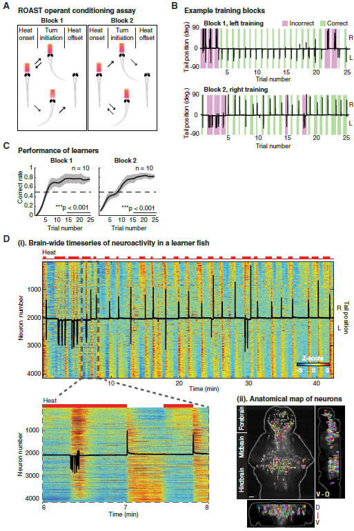
Figure 1.
An operant conditioning assay for larval zebrafish combined with whole-brain calcium imaging.
(A) Relief of Aversive Stimulus by Turn (ROAST). Head-fixed larval zebrafish receive a mildly aversive heat stimulus by an infrared laser (red trapezoid) at the beginning of a trial. The laser is turn...
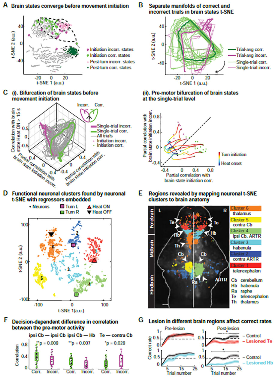
Figure 2.
Decision making relies on coordination and integration of distributed information across the whole brain.
(A) Brain states for a given trial type (correct or incorrect) converge into a smaller region of the t-SNE space before turn initiation (diamonds; incorrect (incorr.): magenta, correct (corr.): green)...
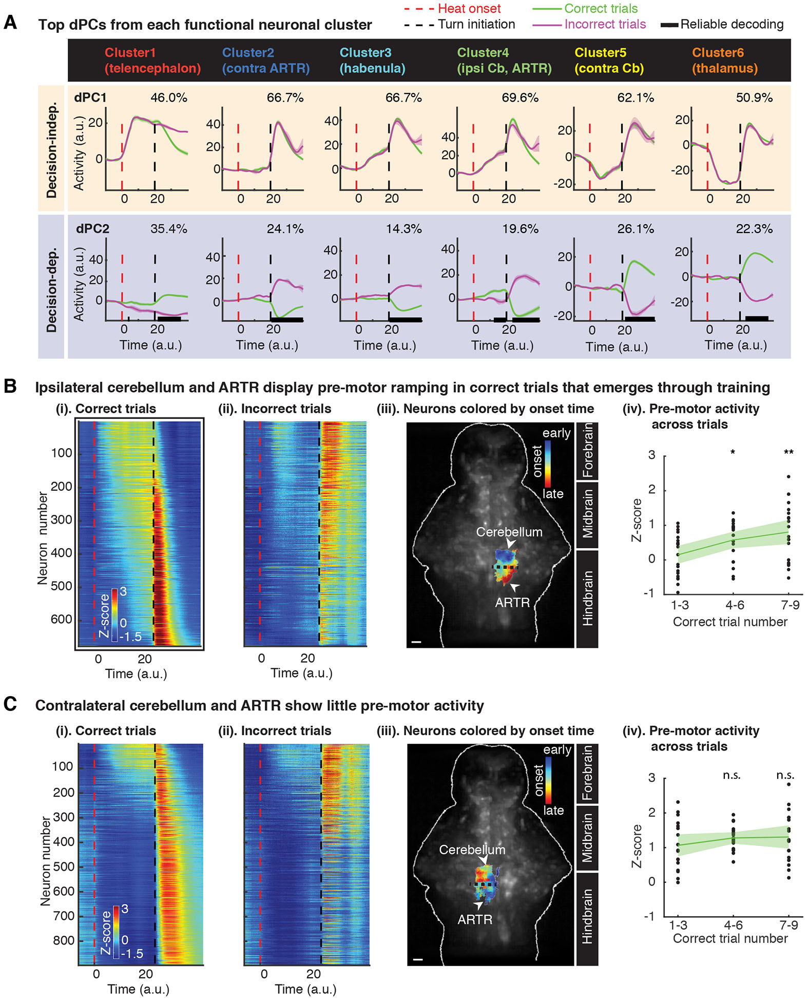
Figure 3.
Preparatory activity in the cerebellum is highly predictive of decision outcome and emerges through training.
(A) Top demixed principal components (dPCs) from each functional neuronal cluster. Population activity from each cluster was projected onto individual dPCs and averaged over trials (lines and shaded b...
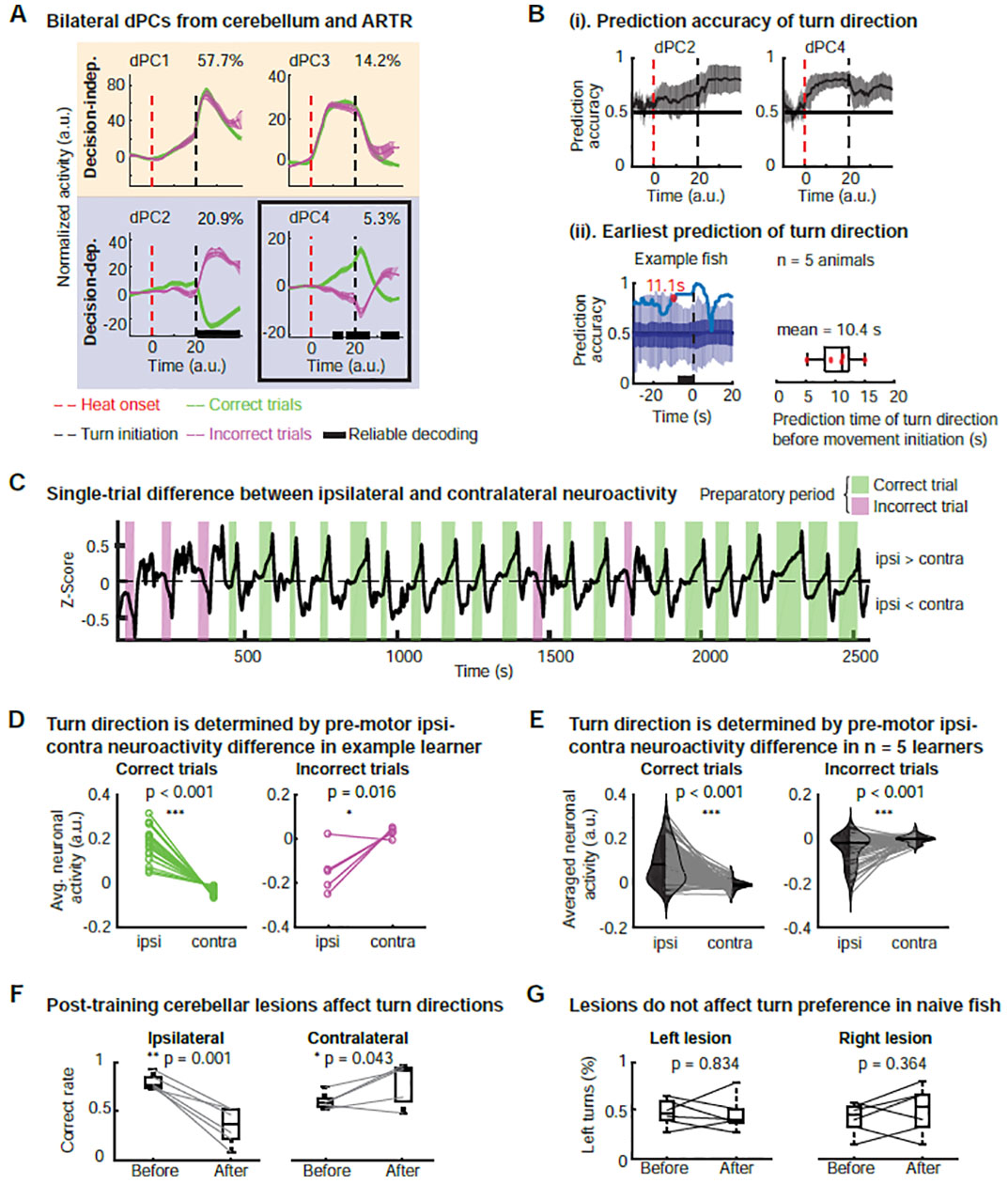
Figure 4.
Bilateral ipsi-contra competition in the cerebellum determines decision outcome.
(A) Bilateral dPCA analysis of joint neuroactivity of cerebellum (Cluster 4 and Cluster 5). Decision-independent dPCs: dPC1 displays pre-motor ramping and post-turn peak; dPC3 displays a plateau shape...
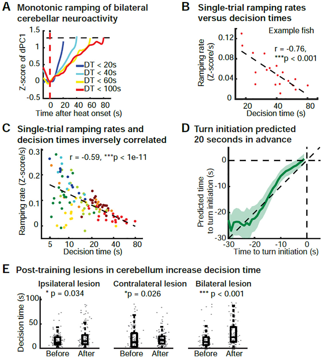
Figure 5.
Bilateral cooperation of cerebellar neuroactivity determines decision time.
(A) Monotonic ramping of bilateral cerebellar population activity grouped by decision time (DT). Turns appear to be initiated when ramping activity reaches a common decision-time-independent threshold...
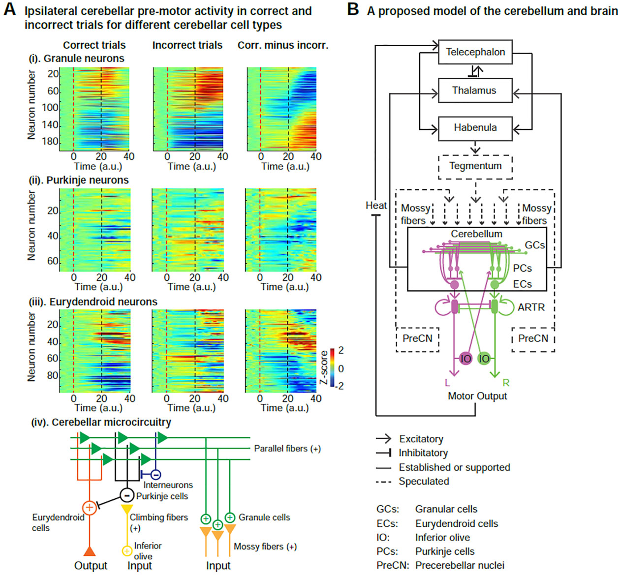
Figure 6.
Proposed model for decision-making network in cerebellum, and the interaction with brain-wide neurodynamics.
(A) Trial-averaged ipsilateral cerebellar activity for different cell types (granule, Purkinje and eurydendroid cells). Dashed line: red for heat onset; black for turn initiation. Only cells showing a...
Figure images are served from the NIH/NLM PubMed Central Open Access Subset or Europe PMC; copyright remains with the publishers and authors.
💬 Discussion
0 commentsNo comments yet. Be the first to start a discussion!
Leave a Comment