Abstract
A straightforward method to achieve super-resolution consists of taking an image sequence of stochastically blinking emitters using a standard wide-field fluorescence microscope. Densely packed single molecules can be distinguished sequentially in time using high-precision localization algorithms (e.g., PALM and STORM) or by analyzing the statistics of the temporal fluctuations (SOFI). In a face-to-face comparison of the two post-processing algorithms, we show that localization-based super-resolution can deliver higher resolution enhancements but imposes significant constraints on the blinking behavior of the probes, which limits its applicability for live-cell imaging. SOFI, on the other hand, works more consistently over different photo-switching kinetics and also delivers information about the specific blinking statistics. Its suitability for low SNR acquisition reveals SOFI's potential as a high-speed super-resolution imaging technique.
🔬 Techniques
✨ Fluorophores
🧪 Sample Preparation
🔬 Cell Lines
🏭 Microscope Brands
🏛️ Research Organizations (ROR)
Affiliated research institutions:
📋 Methods
2.1. Algorithms 2.1.1. SOFI algorithm Initially, SOFI consisted of computing higher-order autocumulants [ 18 ], where the achievable resolution was limited by the effective pixel size of the detector. Recently, it has been shown that this limitation can be circumvented using spatio-temporal cross-cumulants (XC-SOFI) for generating a finer sampling grid. Furthermore, a simple reweighting scheme in the Fourier domain of the n -th order SOFI image has been introduced, which modifies the resulting SOFI PSF to yield the original microscope PSF with an n -fold reduced size, corresponding to a resolution improvement by a factor of n [ 19 ]. Here we implemented those recent developments, calculated spatio-temporal cross-cumulants to generate inter-pixels and estimated the point-spread function, which is necessary for the subsequent Fourier reweighting (FRW). A scheme illustrating the different steps of the SOFI algorithm is depicted in Fig. 1 . The computation of different combinations of spatio-temporal cross-cumulants of each pixel with n -1 of its neighboring pixels enables the construction of an n -fold finer sampling grid in the final image (see Fig. 2 ). Due to the spatial decrease of correlation, the inter-pixels generated by cross-cumulants are lower in amplitude than the pixels generated by the auto-cumulants and thus need to be corrected by a distance factor ( Fig. 1, step 3 ). Using a model (e.g., Gaussian) of the microscope's point-spread function and varying its parameters, these correction factors can be iteratively optimized until all pixels have similar weights. We have used the 2D Laplacian as a cost-function of the optimization algorithm, which turned out to be robust. The resulting estimation of the point-spread function is used in the Fourier reweighting ( Fig. 1, step 4 ). 2.1.2.
Show full methods section
2.1. Algorithms 2.1.1. SOFI algorithm Initially, SOFI consisted of computing higher-order autocumulants [ 18 ], where the achievable resolution was limited by the effective pixel size of the detector. Recently, it has been shown that this limitation can be circumvented using spatio-temporal cross-cumulants (XC-SOFI) for generating a finer sampling grid. Furthermore, a simple reweighting scheme in the Fourier domain of the n -th order SOFI image has been introduced, which modifies the resulting SOFI PSF to yield the original microscope PSF with an n -fold reduced size, corresponding to a resolution improvement by a factor of n [ 19 ]. Here we implemented those recent developments, calculated spatio-temporal cross-cumulants to generate inter-pixels and estimated the point-spread function, which is necessary for the subsequent Fourier reweighting (FRW). A scheme illustrating the different steps of the SOFI algorithm is depicted in Fig. 1 . The computation of different combinations of spatio-temporal cross-cumulants of each pixel with n -1 of its neighboring pixels enables the construction of an n -fold finer sampling grid in the final image (see Fig. 2 ). Due to the spatial decrease of correlation, the inter-pixels generated by cross-cumulants are lower in amplitude than the pixels generated by the auto-cumulants and thus need to be corrected by a distance factor ( Fig. 1, step 3 ). Using a model (e.g., Gaussian) of the microscope's point-spread function and varying its parameters, these correction factors can be iteratively optimized until all pixels have similar weights. We have used the 2D Laplacian as a cost-function of the optimization algorithm, which turned out to be robust. The resulting estimation of the point-spread function is used in the Fourier reweighting ( Fig. 1, step 4 ). 2.1.2.
Localization algorithm
STORM processing, similar to single-molecule tracking algorithms, consists of a frame-by-frame image segmentation and subsequent single-molecule localization using Gaussian fitting [ 22 ]. Figure 3 illustrates the main steps of our implementation. Image segmentation involves filtering with a Laplacian of Gaussian to simultaneously reduce noise and enhance isolated single emitter signals. After threshold background subtraction, the remaining image segments of reasonable sizes are analyzed. The center of gravity of a segment yields a first estimate of the fluorophore's position, which is introduced as an initial value in the Gaussian fit ( Fig. 3, step 2 ). We applied an unweighted least-squares optimization to estimate the amplitude, position, waist and background using the Levenberg-Marquardt algorithm. Estimates of width and amplitude that varied by more than a factor of two from their expected values were discarded to reduce the number of false positives. The estimated single-molecule positions were mapped into a high-resolution image ( Fig. 3, step 3 ). Fig. 1. The different steps of calculating cross-cumulant SOFI with Fourier reweighting (XC-SOFI-FRW), illustrated for the second order. Before the computation of crosscumulants, the mean is subtracted from the data. Using different combinations of crosscumulants between pixels gives rise to an inhomogeneous weight distribution (step 2), which needs to be corrected by a distance factor (step 3). The distance-factor correction also provides an estimation of the system's PSF. Fourier reweighting (FRW) enables the modification of the SOFI equivalent PSF to retrieve the microscope's PSF with an n -fold reduced size (step 4). Higher-order cumulants are computed using the exact formulation described in [ 21 ]. Scale bars: 200 nm . 2.2.
Simulation
Based on a simulation, we investigated the performance of the SOFI and STORM algorithms under the aspects of photo-switching kinetics, labeling density and signal-to-noise ratio. The simulation generates image sequences of randomly blinking fluorophores that are placed arbitrarily on two parallel bands, each 0.04 Airy units wide, at different separation distances. The fluorophore blinking behavior was simulated as a time-continuous Markov process between on and off states using a 100-fold temporal oversampling. The average blinking rate is then given by k = k on k off k on + k off , (1) where k on = τ −1 off denotes the rate at which the fluorophore is transferred from the off state back to the on state and vice versa for k off = τ −1 on . k was fixed to half the sampling rate ( f ) but was not synchronized with the acquisition time intervals. The number of emitted photons per fluorophore followed a Poisson probability-density distribution with an average photon count rate of 9 kHz in the on state. Similar to measurements, a constant background of 40% of the average molecular amplitude and shot noise was added. For simplicity, we used a Gaussian PSF model with a full-width at half-maximum (FWHM) equal to one Airy unit (237 nm; corresponding to a numerical aperture (NA) of 1.49 and an emission wavelength of 580 nm). The pixel size was 100 nm. For computational ease and to limit the length of the image sequences, we applied generally low labeling densities (5−20/ µ m), which allow longer fluorophore on-times with respect to their off-times, i.e., a low rate ratio Fig. 2. Fourth-order cross-cumulant combinations for pixel i with or without repetitions. Different combinations within a neighborhood matrix of i can be used to generate 15 inter-pixels in between the original pixel matrix (ABCD). Combinations leading to the same inter-pixel are averaged. (a) All n -combinations within a 2×2 neighborhood (ABCD) starting with A and allowing for repetitions are computed. This scheme can be expanded easily to any order n . Due to the presence of autocumulants, this method does not suppress shot noise very well unless non-zero time lags are used. (b) The different combinations within a 4×4 neighborhood of pixel i can be used to generate inter-pixels in a circular arrangement (left). By excluding repetitions (autocumulants), shot noise is suppressed much better. For computational reasons, only combinations featuring the shortest sum of distances with respect to their corresponding inter-pixels are considered. By considering more combinations and averaging over the corresponding cross-cumulants, even more noise could be eliminated. Further simplification can be done by considering only combinations leading to the 15 inter-pixels within ABCD (right). This scheme is expandable until order 10. To go beyond this range, the size of the neighborhood has to be increased. Fig. 3. STORM-principle: The image sequence is processed frame by frame. For the localization, the images are segmented and each isolated diffraction pattern is fitted to a parameterized Gaussian PSF model (step 2). The determined single-molecule positions are combined in a composite image with a ten-fold finer sampling grid (step 3). Scale bars: 200 nm . r = k off k on = τ off τ on . (2) However, we expect the effect to be similar at higher labeling densities if accordingly higher rate ratios and sequence lengths are used. We compared the relative visibility v (in the following referred to as visibility) of the projected line profiles, defined as v 0 = 0.5 I max , 1 − I min I max , 1 + I min + 0.5 I max , 2 − I min I max , 2 + I min (3) v = v 0 ( min { I max , 1 I 1 , I max , 2 I 2 } max { I max , 1 I 1 , I max , 2 I 2 } ) sign { v 0 } , (4) where I max ,1 , I max ,2 , I min , I 1 and I 2 are defined according to Fig. 4 . Fig. 4. The visibility defined in Eq. (4) serves as a benchmark for comparing the different algorithms. The line profiles are obtained by projecting the images along the y direction. I max ,1 and I max ,2 are obtained by taking the mean intensity at the known positions of the lines ( x 1 and x 2 ) and I min is the mean intensity between 0.4( x 1 + x 2 ) and 0.6( x 1 + x 2 ). Scale bars: 500 nm . 2.3. Experiments We used a custom-designed total-internal-reflection fluorescence (TIRF) microscope in epiillumination with an oil-immersion objective (Olympus 60×1.49) and two laser excitation sources.
Fixed human osteosarcoma cells
(U2OS) expressing a β -tubulin-SNAP tag [ 23 ] have been labeled with a photo-switchable probe (BG-Cy3-Cy5) and an imaging buffer containing mercaptoethanol, and an oxygen-scavenging system was used to increase the dark state lifetime of Cy5. All experimental details can be found in [ 24 ].
4. Experimental results The experiments with microtubule structures in human osteosarcoma cells (U2OS) showed significant resolution and contrast enhancements for both STORM and SOFI in comparison to the wide-field image ( Fig. 11 ). Regions of low microtubule density led to well resolved STORM images (e3), whereas the imaging of crossing structures, or regions of high labeling densities, was more problematic due to rarely isolated single emitter patterns (e2). Apparently, the rate ratio was not sufficiently high in these regions. The third order SOFI image reveals the presence of two closely spaced microtubuli at the pointing arrow in (c2). SOFI worked consistently all over the image up to order 3. At higher orders, dimmer and/or weakly fluctuating molecules get lost in the background, and the imaged structures lose connection (see Fig. 11b–11d ). This is mainly due to the fact that SOFI order n raises the heterogeneities in molecular brightness to the power of n , which makes it increasingly difficult to display continuous structures for higher orders without compromising the apparent resolution. The last row in Fig. 11 shows the transversal intensity distributions and FWHMs of a single microtubule, averaged over 400 nm along the structure. Fig. 11. Microtubule structures in human osteosarcoma cells: Experimental demonstration of resolution improvements for SOFI and STORM. Row 2 illustrates the effect of insufficient rate ratios at high labeling densities, which makes it impossible for STORM to resolve the two closely spaced microtubuli at the pointing arrow. Regions of well-separated structures are less problematic (row 3). Row 4 shows the transversal intensity distribution of a microtubule (white box in row 3) fitted to a Gaussian. The intensity distribution is averaged over a length of 400 nm along the structure. Scale bars: 2µm
📊 Figures
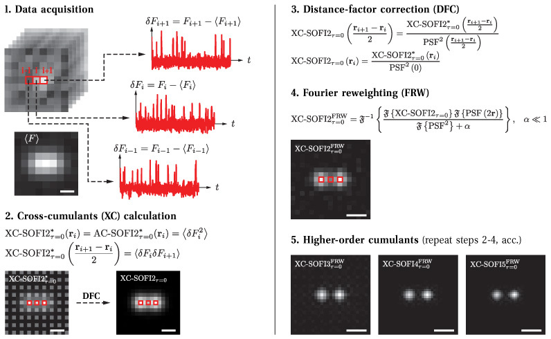
Fig. 1.
The different steps of calculating cross-cumulant SOFI with Fourier reweighting (XC-SOFI-FRW), illustrated for the second order. Before the computation of crosscumulants, the mean is subtracted from t...
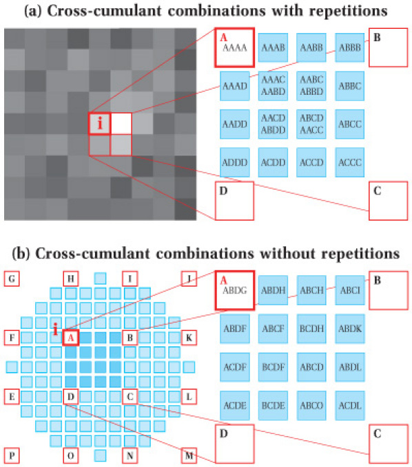
Fig. 2.
Fourth-order cross-cumulant combinations for pixel i with or without repetitions. Different combinations within a neighborhood matrix of i can be used to generate 15 inter-pixels in between the origin...
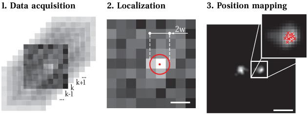
Fig. 3.
STORM-principle: The image sequence is processed frame by frame. For the localization, the images are segmented and each isolated diffraction pattern is fitted to a parameterized Gaussian PSF model (s...
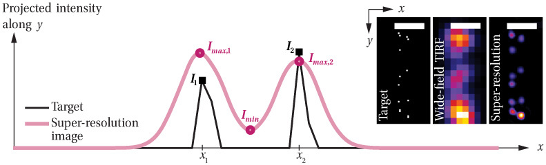
Fig. 4.
The visibility defined in Eq. (4) serves as a benchmark for comparing the different algorithms. The line profiles are obtained by projecting the images along the y direction. I max ,1 and I max ,2 are...
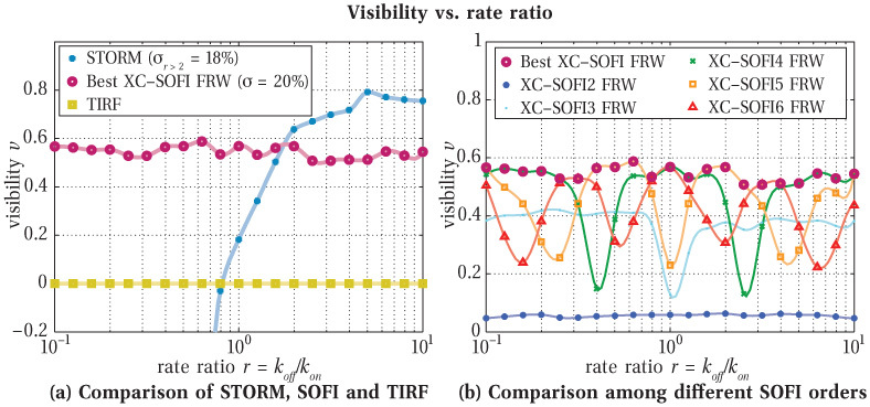
Fig. 5.
Comparison of the visibility versus rate ratio. The best XC-SOFI is obtained by the SOFI order yielding the highest average relative visibility for a specific set of simulation parameters. u03c3 denot...
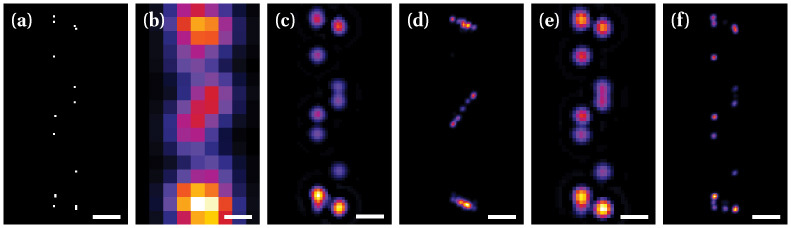
Fig. 6.
Visual comparison of SOFI and STORM reconstructions at different rate-ratios. (a) Target structure. (b) Summed TIRF. (c) XC-SOFI5 FRW, r = 0.6. (d) STORM, r = 0.6. (e) XC-SOFI4 FRW, r = 10. (f) STORM,...
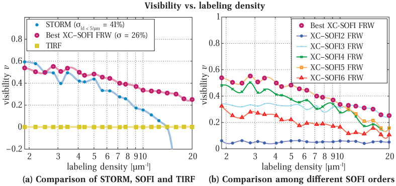
Fig. 7.
Comparison of the visibility versus labeling density. The best XC-SOFI is obtained by the SOFI order yielding the highest average relative visibility for a specific set of simulation parameters. u03c3...
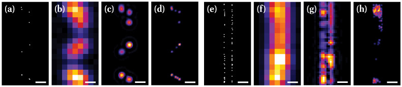
Fig. 8.
Visual comparison of SOFI and STORM reconstructions at different labeling densities. Labeling density: (au2013d) 3/ u00b5 m, (eu2013h) 20/ u00b5 m. (a,e) Target structure. (b,f) Summed TIRF. (c) XC-SO...
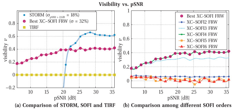
Fig. 9.
Comparison of the visibility versus pSNR. XC-SOFI has been computed using cross-cumulant combinations without repetitions. The best XC-SOFI is obtained by the SOFI order yielding the highest average r...
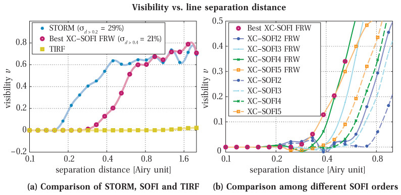
Fig. 10.
Comparison of the visibility versus line separation distance. The best XC-SOFI is obtained by the SOFI order yielding the highest average relative visibility for a specific set of simulation parameter...
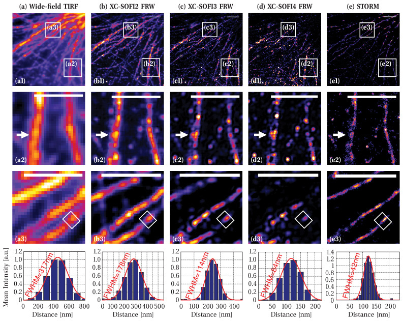
Fig. 11.
Microtubule structures in human osteosarcoma cells: Experimental demonstration of resolution improvements for SOFI and STORM. Row 2 illustrates the effect of insufficient rate ratios at high labeling ...
Figure images are served from the NIH/NLM PubMed Central Open Access Subset or Europe PMC; copyright remains with the publishers and authors.
💬 Discussion
0 commentsNo comments yet. Be the first to start a discussion!
Leave a Comment