Abstract
Transcriptome level expression data connected to the spatial organization of the cells and molecules would allow a comprehensive understanding of how gene expression is connected to the structure and function in the biological systems. The spatial transcriptomics platforms may soon provide such information. However, the current platforms still lack spatial resolution, capture only a fraction of the transcriptome heterogeneity, or lack the throughput for large scale studies. The strengths and weaknesses in current ST platforms and computational solutions need to be taken into account when planning spatial transcriptomics studies. The basis of the computational ST analysis is the solutions developed for single-cell RNA-sequencing data, with advancements taking into account the spatial connectedness of the transcriptomes. The scRNA-seq tools are modified for spatial transcriptomics or new solutions like deep learning-based joint analysis of expression, spatial, and image data are developed to extract biological information in the spatially resolved transcriptomes. The computational ST analysis can reveal remarkable biological insights into spatial patterns of gene expression, cell signaling, and cell type variations in connection with cell type-specific signaling and organization in complex tissues. This review covers the topics that help choosing the platform and computational solutions for spatial transcriptomics research. We focus on the currently available ST methods and platforms and their strengths and limitations. Of the computational solutions, we provide an overview of the analysis steps and tools used in the ST data analysis. The compatibility with the data types and the tools provided by the current ST analysis frameworks are summarized.
🔬 Techniques
✨ Fluorophores
🧪 Sample Preparation
🔬 Cell Lines
🧪 Reagent Suppliers
💻 Software Details
🏛️ Research Organizations (ROR)
Affiliated research institutions:
📋 Methods
2 In situ spatial transcriptomics methods 2.1 Strengths and limitations The sequential single-molecule fluorescent in situ hybridization (sequ-smFISH) and the in situ sequencing (ISS) offer the highest spatial resolution among the ST methods by detecting individual transcript molecules in the samples at the optical resolution of the microscope system ( Table 1 , Fig. 1 A). Of the ST methods, the sequ-smFISH methods have also the highest sensitivity, as they can detect transcripts with over 80% efficiency even when thousands of RNAs are targeted [3] , [6] , [33] , [34] , [35] . However, the in situ ST methods are not quite yet detecting different mRNAs at transcriptome coverage level like the spatial barcoding ST methods based on polyA targeting mRNA capture. A particular strength of in situ ST methods is their exceptional resolution and capture efficiency. The high capture efficiency allows reliable detection of even very lowly expressed transcripts. A targeted design of probe sets focusing on, for example, signaling pathways or transcription and genomic imprinting regulation has proven a great strategy with in situ ST. A prime example of this is a study of the early T cell progenitor development [36] , in which Zhou et al. designed a probe set to analyze the expression of otherwise elusive transcription factors and master regulators expressed in progenitor T cells. In combination with a scRNA-seq, the study was able to provide insight into the synchronized and asynchronized developmental patterns in gene expressions during the early T cell development. The study also elegantly demonstrated the feasibility of sequential use of seqFISH, smFISH, and immunostaining on the same sample. However, it should be noted that the signals from transcripts degrade each FISH cycle [21] setting limits to the number of successive probing rounds and sets the preferential probing order to start from the weakest expressing transcripts. Indicating the power of integration of in situ ST and scRNA-seq methods, seqFISH was used to identify the exact location of scRNA-seq characterized cell types in mouse organogenesis [37] . The Brain Initiative Cell Census Network (BICCN), a collaborative effort to produce reference brain transcriptome atlases is showing in situ ST use in a very large-scale cell mapping project [38] . MERFISH and seqFISH have a single-molecule level resolution which allows analysis of subcellular transcript distributions at the single-cell level adding on top of single-cell transcriptome profiling. The spatial distribution can be used to detect single-cell level features like mRNA targeting, cell polarization, and localization of specific molecular complexes [4] . For functional single-cell transcriptome analysis, the nuclear to cytoplasmic ratio of immature and mature transcripts can be used to infer the regulatory states of genes at the single-cell level through the so-called RNA velocity analysis [33] . RNA velocity data can be used, for example, to construct detailed transcript regulatory profiles and to organize cells to pseudotime trajectories to analyze, for example, cell cycle progression [33] . Showing the use of sequential smFISH at the molecular complex level, Takei et al. resolved the functional architecture of cell nucleus in detail by adapting seqFISH+ method to co-detect localization of 3660 chromosomal loci with 17 functional chromosomal markers, and 70 selected mRNA species [39] . The study indicated a good general correlation between gene activity, localization to different functional nuclear zones, and association of functional chromosomal markers. However, at the single-cell level discordant localization of individual genes with active nuclear zones and the actual transcriptional activity of the genes suggested slower temporal dynamics for a chromosomal spatial organization than for the gene activity regulation. A major limitation with the in situ ST methods is that the optical crowding poses a problem with very high-plexed probe sets as the detection efficiency degrades along with the number of the target mRNAs. This technological limitation is particularly noticeable with ISS methods as the molecular amplification used for signal enhancement increases the optical size of the targets [5] , [6] , [18] . Detection of transcriptome level number of targets would require resolving up to hundreds of thousands of transcripts per cell. The current state-of-the-art seqFISH+ with 60 pseudocolor probe set combined with a clever transcript encoding scheme, optimized sequential probing, and adoption of confocal microscope platform for detection allowed detection of over 30 000 individual transcripts with ∼ 10 000 genes in cultured fibroblasts [4] . The number of simultaneously detected RNA targets in in situ ST is not limited only by the physical limitations set by the used microscopes. The sensitivity of smFISH is based on the number of in situ hybridization probes (ISH) targeting a given gene. For example, seqFISH+ needs the target RNA length to be at least 1 kb to accommodate the in situ hybridization probes for sensitive detection and encoding. This leaves out for example short mRNAs and many other short RNA species including miRNAs from the target repertoire. In MERFISH probes, the use of branched-DNA increased the detection sensitivity of MERFISH technology, and it can now detect even short 100–200 nucleotide long RNA targets with up to 60% efficiency and long RNAs with almost perfect efficiency [20] . This also allows the detection of a dramatically wider variety of RNA species including mRNA alternative splice variants. Remarkably, the increased sensitivity did not increase the optical size of the fluorescent pixel and with adoption of expansion microscope with more sensitive probes Xia et al. were able to measure the expression of around ~10 000 different RNAs simultaneously in cultured cells [33] . The ISS-based ST methods can detect very short RNA species, and the recently published new padlock ligation (PL-lig) based smFISH/ISS ST method BOLORAMIS can detect even miRNAs and single point mutations in cellular RNAs [18] . The sensitivity and specificity of BOLORAMIS and STARmap allow the detection of even different alternative splice forms of transcripts. However, the use of probes to cover transcripts in an untargeted manner is not feasible due to the cost of probes and without a technological leap in microscopy or probe design, the methodology is still limited by the optical crowding. The reverse transcription capture-based ISS methods [40] , [41] can detect RNA molecules in an untargeted manner but due to very low capture efficiency, they detect only a low number of transcripts per cell compared to other ST methods ( Table 1 ). The in situ ST methods are limited also by the speed of the imaging. In both ISS and sequential smFISH, the transcripts are identified by sequentially imaging fluorescence signals using a microscope. Each cycle involves FISH probing or re-probing and imaging steps. The speed of imaging of the multiple FISH cycles with a high-resolution microscope is thus a bottleneck limiting the sample and detection area throughput with the in situ ST methods. The use of 60 pseudocolours for encoding transcripts in seqFISH+ lowered the needed FISH cycles to four (with the included error correction cycle) for theoretical detection of the expression of up to 24 000 genes [4] . This methodological advancement shortened the sample processing time to 1/8th (imaging and hybridization) from the original in seqFISH [34] . Commercial platforms with automated liquid handling and imaging and with the use of optimized probe sets for in situ ST are expected to improve the throughput and increase the availability of in situ ST for researchers.
Show full methods section
2 In situ spatial transcriptomics methods 2.1 Strengths and limitations The sequential single-molecule fluorescent in situ hybridization (sequ-smFISH) and the in situ sequencing (ISS) offer the highest spatial resolution among the ST methods by detecting individual transcript molecules in the samples at the optical resolution of the microscope system ( Table 1 , Fig. 1 A). Of the ST methods, the sequ-smFISH methods have also the highest sensitivity, as they can detect transcripts with over 80% efficiency even when thousands of RNAs are targeted [3] , [6] , [33] , [34] , [35] . However, the in situ ST methods are not quite yet detecting different mRNAs at transcriptome coverage level like the spatial barcoding ST methods based on polyA targeting mRNA capture. A particular strength of in situ ST methods is their exceptional resolution and capture efficiency. The high capture efficiency allows reliable detection of even very lowly expressed transcripts. A targeted design of probe sets focusing on, for example, signaling pathways or transcription and genomic imprinting regulation has proven a great strategy with in situ ST. A prime example of this is a study of the early T cell progenitor development [36] , in which Zhou et al. designed a probe set to analyze the expression of otherwise elusive transcription factors and master regulators expressed in progenitor T cells. In combination with a scRNA-seq, the study was able to provide insight into the synchronized and asynchronized developmental patterns in gene expressions during the early T cell development. The study also elegantly demonstrated the feasibility of sequential use of seqFISH, smFISH, and immunostaining on the same sample. However, it should be noted that the signals from transcripts degrade each FISH cycle [21] setting limits to the number of successive probing rounds and sets the preferential probing order to start from the weakest expressing transcripts. Indicating the power of integration of in situ ST and scRNA-seq methods, seqFISH was used to identify the exact location of scRNA-seq characterized cell types in mouse organogenesis [37] . The Brain Initiative Cell Census Network (BICCN), a collaborative effort to produce reference brain transcriptome atlases is showing in situ ST use in a very large-scale cell mapping project [38] . MERFISH and seqFISH have a single-molecule level resolution which allows analysis of subcellular transcript distributions at the single-cell level adding on top of single-cell transcriptome profiling. The spatial distribution can be used to detect single-cell level features like mRNA targeting, cell polarization, and localization of specific molecular complexes [4] . For functional single-cell transcriptome analysis, the nuclear to cytoplasmic ratio of immature and mature transcripts can be used to infer the regulatory states of genes at the single-cell level through the so-called RNA velocity analysis [33] . RNA velocity data can be used, for example, to construct detailed transcript regulatory profiles and to organize cells to pseudotime trajectories to analyze, for example, cell cycle progression [33] . Showing the use of sequential smFISH at the molecular complex level, Takei et al. resolved the functional architecture of cell nucleus in detail by adapting seqFISH+ method to co-detect localization of 3660 chromosomal loci with 17 functional chromosomal markers, and 70 selected mRNA species [39] . The study indicated a good general correlation between gene activity, localization to different functional nuclear zones, and association of functional chromosomal markers. However, at the single-cell level discordant localization of individual genes with active nuclear zones and the actual transcriptional activity of the genes suggested slower temporal dynamics for a chromosomal spatial organization than for the gene activity regulation. A major limitation with the in situ ST methods is that the optical crowding poses a problem with very high-plexed probe sets as the detection efficiency degrades along with the number of the target mRNAs. This technological limitation is particularly noticeable with ISS methods as the molecular amplification used for signal enhancement increases the optical size of the targets [5] , [6] , [18] . Detection of transcriptome level number of targets would require resolving up to hundreds of thousands of transcripts per cell. The current state-of-the-art seqFISH+ with 60 pseudocolor probe set combined with a clever transcript encoding scheme, optimized sequential probing, and adoption of confocal microscope platform for detection allowed detection of over 30 000 individual transcripts with ∼ 10 000 genes in cultured fibroblasts [4] . The number of simultaneously detected RNA targets in in situ ST is not limited only by the physical limitations set by the used microscopes. The sensitivity of smFISH is based on the number of in situ hybridization probes (ISH) targeting a given gene. For example, seqFISH+ needs the target RNA length to be at least 1 kb to accommodate the in situ hybridization probes for sensitive detection and encoding. This leaves out for example short mRNAs and many other short RNA species including miRNAs from the target repertoire. In MERFISH probes, the use of branched-DNA increased the detection sensitivity of MERFISH technology, and it can now detect even short 100–200 nucleotide long RNA targets with up to 60% efficiency and long RNAs with almost perfect efficiency [20] . This also allows the detection of a dramatically wider variety of RNA species including mRNA alternative splice variants. Remarkably, the increased sensitivity did not increase the optical size of the fluorescent pixel and with adoption of expansion microscope with more sensitive probes Xia et al. were able to measure the expression of around ~10 000 different RNAs simultaneously in cultured cells [33] . The ISS-based ST methods can detect very short RNA species, and the recently published new padlock ligation (PL-lig) based smFISH/ISS ST method BOLORAMIS can detect even miRNAs and single point mutations in cellular RNAs [18] . The sensitivity and specificity of BOLORAMIS and STARmap allow the detection of even different alternative splice forms of transcripts. However, the use of probes to cover transcripts in an untargeted manner is not feasible due to the cost of probes and without a technological leap in microscopy or probe design, the methodology is still limited by the optical crowding. The reverse transcription capture-based ISS methods [40] , [41] can detect RNA molecules in an untargeted manner but due to very low capture efficiency, they detect only a low number of transcripts per cell compared to other ST methods ( Table 1 ). The in situ ST methods are limited also by the speed of the imaging. In both ISS and sequential smFISH, the transcripts are identified by sequentially imaging fluorescence signals using a microscope. Each cycle involves FISH probing or re-probing and imaging steps. The speed of imaging of the multiple FISH cycles with a high-resolution microscope is thus a bottleneck limiting the sample and detection area throughput with the in situ ST methods. The use of 60 pseudocolours for encoding transcripts in seqFISH+ lowered the needed FISH cycles to four (with the included error correction cycle) for theoretical detection of the expression of up to 24 000 genes [4] . This methodological advancement shortened the sample processing time to 1/8th (imaging and hybridization) from the original in seqFISH [34] . Commercial platforms with automated liquid handling and imaging and with the use of optimized probe sets for in situ ST are expected to improve the throughput and increase the availability of in situ ST for researchers.
Specific data processing steps with ST
Deriving cell-by-gene and cell-by-location matrices for ST analysis from the large set of raw in situ microscopy image data takes several computational steps. For example, in a 69-bit 10 000 gene MERFISH experiment, for each of 256 tiled fields of views (FOV), 23 rounds of three color fluorescent images were taken at six different focal z-planes with an additional single image at fiducial bead z-plane [33] . This is 111 872 single-channel microscope images to process into a form that can be used to extract 69-bit transcript codes and locations to construct cellular transcriptome profiles. This section covers the in situ ST-specific data analysis steps from the raw image data to the spatial cell type pattern analysis. The more advanced analysis steps commonly used with many ST dataset types are covered in Section 5 .
Preprocessing and spot registration
The probed transcripts show in raw images as signal spots that, due to limitations in automated microscopy imaging and due to chromatic aberrations, are not necessarily in the same position (in register) in the sequentially imaged FOVs ( Fig. 2 A). Therefore, the images in each FOV are aligned using cross-correlation of the fiducial marker peak signals or nuclear stains ( Fig. 2 B) [4] , [6] , [42] . Usually, the signal aligning and enhancing steps also include chromatic aberration and illumination correction with microscope setup specific control images, image deconvolution, and background subtraction [43] . For a composite representation of the whole imaged sample, the single or multi-channel FOVs can be stitched together with a process guided by the overlaps in the FOV tiles [28] , [44] . Fig. 2 Preprocessing of raw in situ image data. A) Image alignment is required since the corresponding signal spots in raw images from sequential probing and imaging cycles (img1, img2, img3) are not in the register in shared Euclidean space. To align the spots, the images are moved and rotated in relation to each other. B) In the aligned sequential data, the corresponding signal spots are in the register in the whole image stack, and they form the sequ-FISH barcode. C) Cell segmentation assigns every location in the image to defined cells, nuclei, or background. Transcripts are assigned to cells based on their spatial coordinates in relation to cell mask coordinates. Cells are also assigned with spatial coordinates (X, Y) in the same Euclidean space. D) Connected strings of signal spots, which are called from the image stack in panel B, are the barcodes to identify the transcript/gene at that particular coordinate location (left). The gene identities are decoded from the barcodes and counted into the cell with an overlapping coordinate location in the cell to gene matrix (right). In aligned images, each positive spot/pixel/voxel is a potential transcript, with a location in the pixel coordinate system and transcript identifier encoded by the levels of the sequential image channels. The transcript spots are called by finding the local maxima of the images and by selecting the values that are above a certain pixel threshold [45] . The barcodes are then extracted as per location signal strings for decoding ( Fig. 2 D) [3] , [42] . Details of the above steps and the barcode decoding with error correction and spot quality control (QC) heavily depend on the used microscope setup and in sit u ST method (MERFISH, seqFISH or ISS). Readers interested in these details are referred to the procedures explained in the original research referenced in Table 1 . The decoded transcripts are arranged into a gene-by-location matrix containing the identifiers and 2D or 3D location of every identified transcript in the used coordinate system.
Spatial segmentation
To construct single-cell or other spatial unit transcript profiles in the sample, segmentation and counting steps are performed to assign the detected transcripts into desired functional spatial units. Segmentation masks defining coordinates of the spatial units are done by tracing the shapes of the targeted features from the acquired images or algorithmically with the spatial distribution of the transcripts ( Fig. 2 C). Reflecting the challenges in the segmentation of different biological samples, several different computational methods and strategies have been developed for segmentation. These start from simple manual segmentation by marker thresholding and end with various automated machine learning utilizing strategies [43] . In a standard cell segmentation, the specific markers are used to divide the FOV area into nuclear, cytoplasmic, and empty regions. The individual cells are delineated by selecting the nuclei of each cell as a center and then propagating the cytoplasmic area around the nuclei. Different computational methods are employed to estimate the extent and shape of cell boundaries mathematically or by using marker signals or both. The various machine learning-based segmentation tools, like U-net [46] , DeepCell [47] , Mesmer [48] , and CellPose [49] , use ST images and pre- or post-stain marker data to predict spatial segmentation [50] . In cases where only transcript signals are present, the cell segmentation or segmentation-free cell transcriptome identification relies on algorithms that use spatial transcript distributions [51] or annotated transcript profiles are used in combination with the ST data to jointly segment and annotate the cell types, as in the recent methods SSAM [51] , Baysor [52] , and JSTA [53] . Finally, the identified transcripts within the spatial unit regions are counted based on the segmentation masks to construct the cell-by-gene and cell-by-location matrices for ST data analysis ( Fig. 2 D). The image processing, segmentation, decoding, and counting steps can be performed by scripting with Python, R, or MatLab image processing packages or modules. The Starfish [54] and its fork SMART-Q with multiomics capabilities collect python tools and scripts for building pipelines to process images and get the cell-by-gene and cell-by-location matrices from raw microscope images of different in situ ST methods. Other options offering useful functionalities for image processing, spot calling, and cell segmentation include PySpots [53] , [55] , Cellpose [49] , and FISH-quant [56] in python, and EBImage [57] and imager [58] in R. Of the complete ST data analysis frameworks Squidpy [59] has cell and nuclei segmentation capabilities available ( Table 2 ). Table 2 Spatial data analysis frameworks. Package Giotto Seurat STUtility SPATA2 Squidpy scvi-tools stLearn GeoMx tools Platforms R/Python R R R Python Python Python R Input data ig,mt,lc ig,mt,lc ig,mt,lc ig,mt,lc ig,mt,lc mt,lc ig,mt,lc mt,lc Datacontainer Giotto Seurat Seurat SPATA Adt,img Adt Adt S4 ST data types is,sb is,sb sb is,sb is,sb is,sb is,sb gmx Spatial segmentation • • Nuclei count • QC and preprocessing • • • • • • • • Descriptive statistics • • • • • • • • Dimensionality reduction • • • • • • • • • • • • • • • • • • • • • • • • • • • • • • • • • • • Cell/spot clustering • • • • • • • • • • • • • • • • • • • • • • • • • • • • Data visualizations • • • • • • • • Factor analysis • • Differential expression • • • • • • • • Cell type annotation • • Deconvolution • • • • • • • • • Reverse deconvolution • Cell type signature inference • • Spatial representations • • • • • • • • • • Genes with spatial patterns • • • • • • • • Spatial domains • • • • Cell neighborhood analysis • • Neighbor dependent genes • Cell–cell interaction • • • Ligand-receptor analysis • • • Intergroup gene expression • • GSEA and GSVA • CNV estimation • Spatial visualization • • • • • • • • Interactive visualization • • • • • • Interactive annotation • • • Image analysis • • • Features extraction images • Deep learning analysis • • • Cell trajectory analysis • • Note: Each dot represents single method for the task. Squidpy and scvi are build on top of Scanpy. Table 2 abbreviations see 2.
3 Spatial barcoding methods 3.1 Strengths and limitations Spatial barcoding ST methods are based on the limited diffusion of the target RNA molecules and their capture by the position-indicating barcoded DNA-oligos ( Fig. 1B-C ). Compared to in situ ST methods, spatial barcoding ST excels in availability, simplicity, and untargeted mRNA capture 1 . Nonetheless, it is behind in resolution and capture efficiency compared to many in situ ST methods ( Table 1 ). Both the resolution and capture efficiency in spatial barcoding ST methods have increased gradually since early spot arrays [23] and custom microarrays [63] , in which the center-to-center distance was in the 200 to 100-micron range. In these first-generation arrays, each “spot” captured transcripts from multiple cells, which complicated the cell and spatial data analysis. Recently, the spatial resolution in spatial barcoding arrays has increased to a level of single-cell size and beyond. In Slide-seq, this was obtained by micro ball-arrays [8] , [64] and, in DbiT-Seq, by chips with microchannels injecting the spatial barcode oligos [10] . The spatial barcoding reached the subcellular resolution with high-definition spatial transcriptomics (HDST) oligo arrays [9] . The highest resolution and the best capture efficiencies have so far been achieved with Seq-Scope, Stereo-Seq, and Pixel-seq [7] , [24] , [25] . These recent high-resolution and high-density DNA-oligo spatial barcoding arrays not only increased the resolution to the sub-micron level, but the mRNA capture efficiency has also improved to a comparable level with the droplet-based scRNA-seq methods ( Table 1 ). This allows robust untargeted detection of medium expression level genes at the single-cell level and even between the cellular compartments. The HDST and Seq-Scope studies demonstrated that the high-resolution arrays can locate even rare cell types and resolve the gene expression differences at subcellular resolution, which makes for example the nuclear-to-cytoplasmic type of RNA-velocity of analysis feasible for spatial barcode ST methods [9] , [25] . The preprints showcase the capabilities and limitations of Stereo-Seq with tumor leading-edge samples [65] and high-resolution spatial transcriptome atlases produced from regenerating axolotl brains and the developmental stages of the mouse, zebrafish, and fruit fly embryos [7] , [66] , [67] , [68] . Already these detailed transcriptome atlases, after being released into the public domain, could provide a rich resource of transcriptomic data to analyze the developmental process and brain regeneration of multicellular organisms. It will also be a great resource for testing and developing bioinformatics, data storage, and data handling methods for the analysis of such large spatial transcriptomics datasets. The high-density spatial barcoding arrays are a big developmental step towards a universal method in ST, even though the Seq-Scope, Stereo-seq, Pixel-seq, HDST, and DbiT-Seq are still behind in resolution and capture efficiency compared to the in situ ST methods. However, wide adoption of high-density spatial barcoding arrays may be bottlenecked by the array production and array indexing as these require special techniques like customized use of Illumina sequencer [7] , custom microchip production [10] , or highly optimized arraying of oligos on to a polyacrylamide gel matrix [24] . Even though the state-of-the-art spatial barcoding methods are not yet widely available, they have shown that the fast pace in the development of ST is still going on strong and that by optimizing spatial barcoding, it is possible to acquire untargeted high gene coverage subcellular resolution data. The latest high-density spatial barcode arrays are not yet generally available for researchers, and hence only pioneering studies have been published. Nonetheless, the spatial barcoding methods with lower resolution arrays have been available for some time and several studies have indicated their power for biological discoveries. The lower resolution spatial barcoding methods have been successfully used to dissect regional gene expression profiles in homeostatic tissues and developmental settings. For example, Slide-seq was used to produce an ST atlas of the mouse testis to decipher the complex organization of mammalian spermatogenesis at an unprecedented level [69] . The spatial transcriptomics with different pattern detection algorithms has allowed a detailed characterization of the normal gut functions and the functions in inflammatory disease [70] , [71] . The spatial transcriptomics has also revealed many novel features in various tumor samples [63] , [72] , [73] , [74] , [75] . These studies have, for example, revealed regional enrichment patterns for cancer cell subtypes and co-enrichments of cancer cells with different subtypes of non-malignant cells [63] . These regional gene expression patterns in turn help to identify candidate signaling pathways and mechanistic interactions between cancer, stromal, and immune cells and to identify prognostic markers [76] , [77] .
Specific data processing steps with spatial barcoding ST
In spatial barcoding, the transcript and the location data are in a DNA format. The sequencing step converts this into a digital format that can be processed computationally. This section covers the spatial barcoding-specific data analysis steps from the raw sequence data to the spatial cell type pattern analysis. The more advanced analysis steps commonly used with many ST dataset types are covered in Section 5 .
Preprocessing and location matrix generation
The preprocessing steps of the spatial barcoding raw sequence data are relatively straightforward and similar to scRNA-seq data. In spatial transcriptomics, instead of a gene to droplet barcode matrix, a gene to spot matrix is generated. The information to build the gene expression (transcript sequences) to spot position (spatial barcodes) matrix is in the paired-end sequencing reads. To identify the expressed genes, the sequences are aligned against an annotated reference genome using, for instance, STAR aligner [78] or Kallisto pseudo-aligner [79] . A second alignment step against a decoy genome can be used to filter out unwanted contaminating sequences [80] . Each sequence pair also contains the spatial barcode sequence and a unique molecular identifier (UMI), which is used to remove the PCR copies of the captured transcripts arising during sequencing library preparation. The expression levels of the genes are counted from the deduplicated, aligned, and barcode-associated reads, and a spatial barcode-by-gene matrix is generated (analogous to Fig. 2 D). STARsolo [81] , bustools [79] , ST Pipeline [80] , Spaceranger count, and Slide-seq/drop-seq tools [69] , [82] are commonly used solutions to produce the spatial barcode-by-gene matrix. The spatial barcode-by-location data connects each transcript to a location coordinate in the sample. The coordinates are used to construct spatial relationship graphs and grids for the spot or cell interconnection analyses, assign transcripts to cells after segmentation with subcellular resolution data, and for visualizations and joint analyses of the spots and different features on the associated tissue images. For instance, in the Visium platform, the barcode sequences and their positions in the spatial grid are fixed and the Spaceranger count creates a barcode-by-location matrix for spatial analyses. In spatial barcode methods with stochastic barcode spot locations, the spot barcode-by-location matrix is constructed in method-specific array sequencing and indexing step [7] , [8] , [9] , [24] , [25] . To visualize or jointly analyze transcripts with tissue images, the barcode coordinate system needs to be aligned with the one used with the tissue images. The Spaceranger count detects the spot positions (fiducial detection) from the bright-field image and creates data for the spot-image alignment. The spatial barcode-spot alignment with the images can also be done interactively [7] , [9] or by using custom scripts [8] .
Estimation of the spot-wise cell type compositions
The spatial barcoding will locate the transcripts at multi- or subcellular spatial resolution. In multicellular resolution spatial barcoding, each spot can contain transcripts from multiple cells. The cell compositions and regional enrichment of different cell types and cell stages in the spots can be resolved with computational deconvolution, mapping, enrichment, and data-integration-based methods [83] , [84] . For instance, SPOTlight [85] uses non-negative matrix factorization (NNMF) and SpatialDecon [86] log-normal regression for deconvolution of the transcriptomics data, whereas Cell2Location is based on a Bayesian model [87] and Tangram is a deep learning framework to resolve cell types. The ST-framework Giotto (discussed in section 5.1.) uses enrichment-based options for cell type composition analysis [88] and Seurat anchor-based integration [89] . The spot compositions are reported as cell type proportions or probabilities of occurrence in the spot. The latest deconvolution methods can also report the estimated transcriptomes of the identified cell types. Most deconvolution methods use annotated reference transcriptome profiles derived from scRNA-seq or bulk RNA-seq datasets, making the accuracy and resolution of the cell type identification highly dependent on the compatibility of the used reference profiles with the cells in the target sample. However, the recently published conditional autoregressive-based deconvolution (CARD) [90] and the latent Dirichlet allocation based STdeconvolve [91] offer reference-free deconvolution methods, which is useful when optimal reference scRNA-seq profiles are not available.
Spatial segmentation
The objective of segmentation is to construct masks to assign the detected transcripts to individual cells, nuclei, or larger objects. The segmentation with spatial barcoding data is essentially the same process as with in situ based ST methods and is based on the stained image data of the target tissue in combination with the actual gene signals. Usually, ST data have associated image data with hematoxylin and eosin (H&E) staining, indicating the location of nuclei and selected structural features. In some cases, fluorescent staining for different cellular markers is available to guide the segmentation. Despite intense development, the segmentation of tissues with densely packed cells is still one of the most challenging steps in the analysis of spatial data. The decisions for segmentation strategy and methods depend heavily on the sample type, the platform used, and the available data to guide the segmentation. Several methods varying from manual assignment to statistical, supervised, semi-supervised, and unsupervised machine learning applications have been developed for the task with other data types (see in situ ST data segmentation). So far, the high-resolution spatial barcoding transcriptomics has not been widely available, and a simple grid segmentation has been used in some of the studies [7] , [65] . We anticipate the development of deep learning models for feature segmentation and cell type identification with the large spatial barcoding ST datasets.
4 Regional selection spatial transcriptomics methods Laser capture microdissection coupled with RNA-sequencing (LCM-seq) and digital spatial profiling (DSP) are methods that use flexible regions of interest (ROI) binning in spatial transcriptomics [14] , [15] , [16] , [17] . Each selection bin contains transcripts from one ROI and they are barcoded for backtracking of the location in the sample. After sequencing and processing, the bins are used similarly to the spots in spatial barcoding arrays, except for that the regions can vary in size, shape, and can be discontinuous ( Fig. 1 D). Depending on the researchers’ choices, each bin can contain transcripts from one or more cells and the ROIs can be selected, for example, to be homogenous in size and shape, cell type, cell marker, or consist of a functional region in the sample [14] , [92] .
Strengths and limitations
Recently the DSP, under the commercial name GeoMx, has gained popularity as a nearly whole transcriptome level ST method with flexible ROI selection that works also with FFPE samples. In GeoMx, the samples are hybridized with analyte probes detecting RNA or proteins, which upon laser illumination release their oligonucleotide tags with the identifiers of the target transcripts or proteins. The oligonucleotide tags are collected after each round of illumination and enzymatically barcoded for the collection bin identification. In LCM-seq the transcripts collected to each bin are barcoded by using barcoded DNA-oligos in reverse transcription reaction. In both methods, a DNA library containing the pooled bins is sequenced and the transcript count-to-bin matrix is resolved. In GeoMx up to four fluorescent markers can be used to guide the sampling or ROIs can be selected based on the physical properties of the sample like distance from the feature of interest and/or by following the shape of the biological unit of interest. In LCM-seq the choice of selection markers depends on the used LCM-seq instrument. The strategies for ROI selection/sampling vary and are decided by the researcher based on prior knowledge and suitability for the research setting [14] , [92] . The flexible sampling allows the development of complex sampling strategies including for example selection of cell type-specific ROIs for profiling and then use of these in deconvolution of the mixed cell ROIs in the same sample. The available data analysis options are limited by the sampling strategy, hence the markers and the cell pooling to bins at the sampling phase should be carefully thought out before the experimental phase [92] . The spatial resolution of the GeoMx and LCM-seq data is determined by the sampling plan. The ROIs can be as small as single cells; however, the throughput in GeoMx and LCM-seq does not allow single-cell analysis on a scale comparable to in situ or spatial barcoding ST methods. GeoMx is also limited by the reliable quantification of transcripts, which in DSP requires 20 to 300 cells per ROI [14] and is thus below the current other ST methods. The transcript detection efficiency in LCM-seq depends on the sequencing library generation method and can be at the highest on the level with tube-based scRNA-seq. GeoMx does not offer untargeted mRNA capture like LCM-seq and spatial barcoding ST. The largest currently available pre-designed probe sets for GeoMx can detect over 18,000 protein-coding genes with a possibility for customization and co-detection of a number of protein targets. An advantage of the GeoMx probing protocol is that it is minimally destructive, and the tissue slides may be used for other applications like H&E staining or immunohistochemistry for retrieving additional information [14] . The GeoMx can shine in the analysis of sample cohorts in which only a limited number of biological compartments or cell types need to be sampled to answer the research questions. For example, GeoMx DSP results have revealed spatial heterogeneity in gene profiles in the host response to SARS-CoV-2 infection in lung samples [93] . DSP has also been used to profile diabetic foot ulcers [94] , detect alterations in diabetic kidneys [95] , and analyze intra-tumor and inter-tumor heterogeneity in various tumor types [96] , [97] , [98] , [99] . With the aid of deconvolution, GeoMx data was used to estimate cell level heterogeneity of tumor-infiltrating lymphocytes in different tumor microenvironments [86] . LCM-seq showed its usability in a study where neurons were collected from different regions of the brainstem and spinal cord for the identification of genes protecting neurons from spinal muscular atrophy associated cell death [100] .
Specific data processing steps with regional selection ST
The cells or regions for analysis are usually pooled at the ROI selection phase in GeoMx and LCM-seq either due to detection efficiency or throughput limitations. Unless carefully sampled, the ROIs will have cells in different stages or consist of heterogeneous cell types. Hence, the analysis depends heavily on the choices taken at ROI selection. In its simplest form, the transcriptomic profiles of GeoMx and LCM-seq ROIs are compared to each other to identify differentially expressed genes. GeoMx proprietary analysis software offers tools for basic analysis. For custom analysis, the GeoMx data can be converted from proprietary file formats to the more accessible spatial data format with the GeoMx tools package in R, which offers the capability for filtering ROIs and probes with quality control parameters associated with sequencing, alignment, and negative control probes included in the pre-designed probe sets. The GeoMx tools package also includes tools for normalization, dimensionality reduction, clustering, differential gene expression analysis, and options for visualization, such as UMAP, t-SNE, and volcano plots. Like spatial barcoding ST data, the GeoMx and LCM-seq multicell ROIs can be analyzed for cell compositions with deconvolution tools, such as the SpatialDecon R package for constrained log-normal regression-based deconvolution of GeoMx and other ST data [86] . For cell type prediction SpatialDecon uses provided cell type signatures or custom ones that can be inferred from RNAseq and scRNA-seq datasets. It can also form new cell profiles “on the fly” from pure cell ROIs and use tumor cell-type-specific ROIs to identify confusing genes in the target cell profiles to aid deconvolution of non-tumor cell types. To enhance estimates, SpatialDecon uses background counts of decoy probes and can also use nuclei counts to estimate total cell counts. For neighborhood analysis, the SpatialDecon includes tools to model the gene expression profiles and up and downregulation of genes in ROIs by using the estimated cell counts with a so-called reverse deconvolution method. Additional computational analyses can be done with custom scripts or other available ST-tools after the conversion of data to a suitable format. However, advanced analysis using spatial relationships (see Section 5 ) can be performed with the GeoMx and LCM-seq spatial datasets only if the spatial coordinates are resolved for the ROIs.
📊 Figures
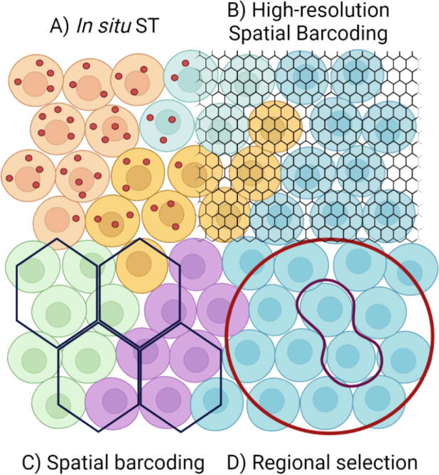
Fig. 1
Spatial transcriptomics methods produce data at different spatial resolutions. A) In situ ST methods detect selected targets at single-molecule resolution in their original location. Spatial informati...
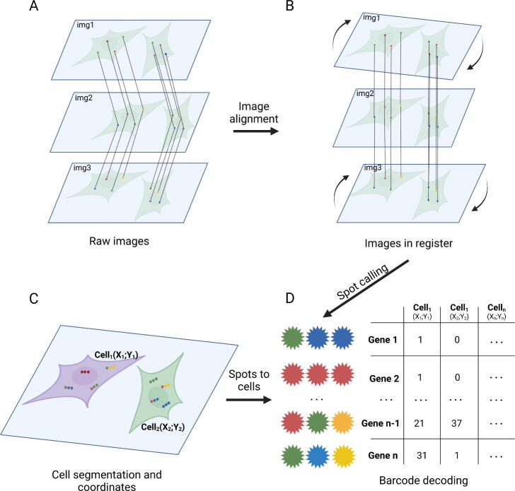
Fig. 2
Preprocessing of raw in situ image data. A) Image alignment is required since the corresponding signal spots in raw images from sequential probing and imaging cycles (img1, img2, img3) are not in the ...
Fig. 3
Overview of the information that may be extracted from spatial transcriptomics data. A) Overall cell type distribution in tissue space shows specialized cell type patterns that reflect communal functi...
Figure images are served from the NIH/NLM PubMed Central Open Access Subset or Europe PMC; copyright remains with the publishers and authors.
💬 Discussion
0 commentsNo comments yet. Be the first to start a discussion!
Leave a Comment