Abstract
Sensory information is translated into ensemble representations by various populations of projection neurons in brain circuits. The dynamics of ensemble representations formed by distinct channels of output neurons in diverse behavioral contexts remains largely unknown. We studied the two output neuron layers in the olfactory bulb (OB), mitral and tufted cells, using chronic two-photon calcium imaging in awake mice. Both output populations displayed similar odor response profiles. During passive sensory experience, both populations showed reorganization of ensemble odor representations yet stable pattern separation across days. Intriguingly, during active odor discrimination learning, mitral but not tufted cells exhibited improved pattern separation, although both populations showed reorganization of ensemble representations. An olfactory circuitry model suggests that cortical feedback on OB interneurons can trigger both forms of plasticity. In conclusion, we show that different OB output layers display unique context-dependent long-term ensemble plasticity, allowing parallel transfer of non-redundant sensory information to downstream centers. VIDEO ABSTRACT.
🔬 Techniques
💻 Software
✨ Fluorophores
🧪 Sample Preparation
🏭 Microscope Brands
🧪 Reagent Suppliers
🔴 Lasers
💻 Software Details
💻 Code & Software
💾 Data Repositories
🏛️ Research Organizations (ROR)
Affiliated research institutions:
📋 Methods
Key Resources Table
REAGENT or RESOURCE SOURCE IDENTIFIER Chemicals, Peptides, and Recombinant Proteins 3-Hexanone Sigma-Aldrich Cat#103020 Amyl acetate Sigma-Aldrich Cat#109584 Butyric acid Sigma-Aldrich Cat#B103500 (−)-Carvone Sigma-Aldrich Cat#124931 Ethyl butyrate Sigma-Aldrich Cat# E15701 Ethyl valerate Sigma-Aldrich Cat#290866 Hexanal Sigma-Aldrich Cat#115606 Methyl benzoate Sigma-Aldrich Cat#12460 Methyl valerate Sigma-Aldrich Cat#148997 Valeric acid Sigma-Aldrich Cat#240370 Tamoxifen Sigma-Aldrich Cat#T5648 Midazolam Roche N/A Medetomidine Orion Pharma N/A Fentanyl Sintetica N/A Dexamethasone Mepha Pharma N/A Carbostesin AstraZeneca N/A Flumazenil Roche N/A Naloxone OrPha Swiss N/A Atipamezole Graeub N/A Carprofen Pfizer N/A Experimental Models: Organisms/Strains Mouse: Tg(Pcdh21-cre/ERT)CYoko Yonekura and Yokoi, 2008 RRID: MGI:5140844 Mouse: B6;129S-Gt(ROSA)26Sortm38(CAG-GCaMP3)Hze/J The Jackson Laboratory RRID: IMSR_JAX:014538 Recombinant DNA AAV9.Syn.Flex.GCaMP3.WPRE.SV40 Tian et al., 2009 ; University of Pennsylvania Vector Core N/A AAV9.Syn.Flex.GCaMP6s.WPRE.SV40 Chen et al., 2013b ; University of Pennsylvania Vector Core N/A Software and Algorithms Moco Dubbs et al., 2016 https://github.com/NTCColumbia/moco Contact for Reagent and Resource Sharing Further information and requests for reagents may be directed to, and will be fulfilled by the corresponding author, Dr. Alan Carleton ( alan.carleton@unige.ch ).
Experimental Model and Subject Details
All animal protocols were in accordance with the Swiss Federal Act on Animal Protection and the Swiss Animal Protection Ordinance, and were approved by the University of Geneva and Geneva state ethics committees (authorization numbers: 1007/3387/2, 1007/3758/2 and GE/156/14). Experiments were performed on 2-6 month-old male mice of the following genotype: Pcdh21-CreER hemizygous transgenic mice ( Yonekura and Yokoi, 2008 ), or Pcdh21-CreER hemizygous transgenic mice crossed with Ai38 R26LSL-GCaMP3 homozygous transgenic mice (JAX no 014538; Zariwala et al., 2012 ). Mice were housed in groups of 2–5 in a temperature- and humidity-controlled animal facility (12-h light/dark cycles). All animals were naive to procedures at the beginning of the experiment. Animals were randomly assigned to the various experimental groups.
Show full methods section
Key Resources Table
REAGENT or RESOURCE SOURCE IDENTIFIER Chemicals, Peptides, and Recombinant Proteins 3-Hexanone Sigma-Aldrich Cat#103020 Amyl acetate Sigma-Aldrich Cat#109584 Butyric acid Sigma-Aldrich Cat#B103500 (−)-Carvone Sigma-Aldrich Cat#124931 Ethyl butyrate Sigma-Aldrich Cat# E15701 Ethyl valerate Sigma-Aldrich Cat#290866 Hexanal Sigma-Aldrich Cat#115606 Methyl benzoate Sigma-Aldrich Cat#12460 Methyl valerate Sigma-Aldrich Cat#148997 Valeric acid Sigma-Aldrich Cat#240370 Tamoxifen Sigma-Aldrich Cat#T5648 Midazolam Roche N/A Medetomidine Orion Pharma N/A Fentanyl Sintetica N/A Dexamethasone Mepha Pharma N/A Carbostesin AstraZeneca N/A Flumazenil Roche N/A Naloxone OrPha Swiss N/A Atipamezole Graeub N/A Carprofen Pfizer N/A Experimental Models: Organisms/Strains Mouse: Tg(Pcdh21-cre/ERT)CYoko Yonekura and Yokoi, 2008 RRID: MGI:5140844 Mouse: B6;129S-Gt(ROSA)26Sortm38(CAG-GCaMP3)Hze/J The Jackson Laboratory RRID: IMSR_JAX:014538 Recombinant DNA AAV9.Syn.Flex.GCaMP3.WPRE.SV40 Tian et al., 2009 ; University of Pennsylvania Vector Core N/A AAV9.Syn.Flex.GCaMP6s.WPRE.SV40 Chen et al., 2013b ; University of Pennsylvania Vector Core N/A Software and Algorithms Moco Dubbs et al., 2016 https://github.com/NTCColumbia/moco Contact for Reagent and Resource Sharing Further information and requests for reagents may be directed to, and will be fulfilled by the corresponding author, Dr. Alan Carleton ( alan.carleton@unige.ch ).
Experimental Model and Subject Details
All animal protocols were in accordance with the Swiss Federal Act on Animal Protection and the Swiss Animal Protection Ordinance, and were approved by the University of Geneva and Geneva state ethics committees (authorization numbers: 1007/3387/2, 1007/3758/2 and GE/156/14). Experiments were performed on 2-6 month-old male mice of the following genotype: Pcdh21-CreER hemizygous transgenic mice ( Yonekura and Yokoi, 2008 ), or Pcdh21-CreER hemizygous transgenic mice crossed with Ai38 R26LSL-GCaMP3 homozygous transgenic mice (JAX no 014538; Zariwala et al., 2012 ). Mice were housed in groups of 2–5 in a temperature- and humidity-controlled animal facility (12-h light/dark cycles). All animals were naive to procedures at the beginning of the experiment. Animals were randomly assigned to the various experimental groups.
Method Details Animal preparation
Prior to surgery, animals were anesthetized with an intraperitoneal injection of a mixture containing midazolam (8 mg/kg), medetomidine (0.6 mg/kg) and fentanyl (0.02 mg/kg). Dexamethasone (2 mg/kg) was intramuscularly injected to prevent brain swelling. Carbostesin was subcutaneously injected prior to any incision, and the eyes were protected with artificial tears. The body temperature was maintained at ∼37°C using a heating pad (FHC) during surgery. The skin and periosteum overlying the skull was removed and a custom-made head post was firmly attached to the skull with cyanoacrylic glue and dental cement. Craniotomy (ϕ3 mm) was performed over the olfactory bulbs, and a 3 mm cover glass was sealed with cyanoacrylic glue and dental cement ( Adam and Mizrahi, 2011 , Goldey et al., 2014 , Holtmaat et al., 2009 ). Anesthesia was reversed by subcutaneous injection of a mixture containing flumazenil (1 mg/kg), naloxone (0.12 mg/kg) and atipamezole (75 mg/kg), and carprofen (5 mg/kg) was intraperitoneally injected for analgesia. All mice were allowed to recover for > 7 days after surgery and then habituated to be head restrained > 15 min/day for > 5 days. All experiments were done during daytime. Experiments were terminated when the clarity of the cranial window was not maintained (mostly due to bone regrowth). Expression of genetically encoded Ca 2+ indicator Pcdh21-CreER hemizygous transgenic mice ( Yonekura and Yokoi, 2008 ) were either 1) injected with Cre-dependent recombinant adeno-associated viruses expressing GCaMP3 ( Tian et al., 2009 ) or GCaMP6s ( Chen et al., 2013b ); AAV9.Syn.Flex.GCaMP6s.WPRE.SV40 or AAV9.Syn.Flex.GCaMP3.WPRE.SV40, University of Pennsylvania Vector Core) at least 3 weeks prior to imaging, or 2) crossed with Ai38 R26LSL-GCaMP3 homozygous transgenic mice (JAX no 014538; Zariwala et al., 2012 ) ( Figure 1 a). Only data acquired with GCaMP6s were used for all the figures except Figure S7 . Virus solutions (0.2-0.5 μl) were injected into each hemi-bulb with glass capillaries (tip diameter ∼30 μm) at 250-400 μm below the pial surface. Tamoxifen (50-100 mg/kg) was intraperitoneally injected for 3 consecutive days to induce Cre-mediated recombination, typically one week after virus injection. Two-photon Ca 2+ imaging Imaging was performed with a custom-built two-photon microscope controlled by ScanImage 3.7 ( http://scanimage.vidriotechnologies.com ). Either 20 × (NA0.95, Olympus) or 16 × (NA0.8, Nikon) objective lens was used. Ti-Sapphire laser (Chameleon ultra II, Coherent) was tuned to 910 nm. The fields of view corresponding to ∼340 × 340 μm were imaged at a spatial resolution of 512 × 128 pixels and at a frame rate of 7.81 Hz. Separation of MCs and TCs was based on imaging depth; TCs were imaged in a plane below the glomeruli where cell bodies are embedded within dense neuropil, while MCs were imaged in a deeper plane where cell bodies are clustered in sparser neuropil. This could have led to inclusion of some deep tufted cells in the MC population. Odor application Saturated odorant vapor was diluted 20 times (except for the data in Figure 2 ) with air, and applied for 2 s at a flow rate of 400 sccm with a custom-made olfactometer. Odor application was synchronized to the beginning of inhalation, which was recorded (recorded at 10kHz) with an air pressure sensor placed in front of the other nostril. Odorants used include 3-Hexanone (3H), amyl acetate (AA), butyric acid (BA), (−)-Carvone (C−), ethyl butyrate (EB), ethyl valerate (EV), hexanal (HX), methyl benzoate (MB), methyl valerate (MV), and valeric acid (VA). Odor discrimination task Head-fixed animals were trained to discriminate 2 different binary mixtures of odorants in a lick/no-lick paradigm, as previously described ( Abraham et al., 2012 ). Briefly, animals under water restriction regime (total of ∼1 ml/day for each animal) were subjected to a pre-training protocol followed by a training protocol. The first stage of pre-training protocol aimed to provoke licking of a metal tube. 3 s after a tone (200 ms, 5000Hz) offset, a water drop (2 μl) was unconditionally delivered to animals via a metal tube for ∼20 trials. Licking was detected as the electrical contact of the tube and the tongue of animals, and sampled at 500 Hz. In the second stage of pre-training protocol, 1 s after the tone offset, an odorant ((−)-Carvone) was presented for 2 s, and a water reward was delivered only if animals displayed successful licking, defined by the total duration of licking: odor period was divided into 4 epochs of 500 ms, and the cumulative duration of licking had to be above threshold in more than 1 epoch, which was gradually increased from 40 ms up to 160 ms (40 ms: 30 trials, 80 ms: 30 trials, 120 ms: 30 trials, 160 ms: 100 trials). If animals displayed licking during the pre-odor period (1 s immediately before odor onset), an alternative threshold was used: cumulative licking duration per epoch during the odor period had to be longer than that during the pre-odor period, with the ratio gradually increasing from 100% up to 200% (100%: 30 trials, 125%: 30 trials, 150%: 30 trials, 175%: 50 trials, 200%: 50 trials). Most animals completed the pre-training protocol within 3 days. Animals were then subjected to a training protocol, where they were presented with two binary mixtures of odorants, one being rewarded (S+; AA60EB40) and the other being un-rewarded (S−; AA40EB60). The criteria for correct responses to S+ (‘hits’) were the same as those at the last step of pre-training: successful licking (cumulative licking duration of > 160 ms) in 2 or more epochs during the odor period, or > 200% of cumulative licking duration during the entire odor period compared to the pre-odor period, if any. The criteria for correct responses to S− (‘correct rejection’) were less than 2 epochs with cumulative licking duration of < 80 ms, or < 25% of cumulative licking duration during the entire odor period compared to that during the pre-odor period. No punishment was given to the mice for incorrect trials. Odorants were presented in a pseudo-randomized manner, where the same odor was repeatedly presented in no more than 2 consecutive trials, and the number for each odor was balanced within a block of 10 trials. Inter-trial interval was 20 s, and the number of trials was typically 150 each day per animal.
Computational models
The details of the model are described in our previous work ( Grabska-Barwińska et al., 2017 ). Briefly, our model circuitry consists of four layers and five groups of variables: ORNs, MCs, cortical cells, and two compartments for each cell in the granule cell layer, with firing rates r i m i , c i, g i and g ik respectively. The following equations govern the firing rates of the different cells and thus the dynamics of the system: τ c d c j d t = β j α 0 − c j + β j F j ( c j ) ∑ i γ i − 1 m i 2 w i j τ m d m i d t =− m j 2 v 0 , i + γ i r i − m i ∑ k w i k m g g i k τ g d g i k d t =− g i k + g k w k i g m m i τ g d g k d t =− g k + ∑ j A k j F j ( c j ) where F j ( c j ) ≡ β j e ψ ( c j / β j ) , with ψ the digamma function , β j ≡ β 0 1 + β 0 ∑ i w i j , and w i j = ∑ k w i k m g w k i g m A k j . Here w i j is the weight corresponding to the activation of the the i-th ORN by odor and ν 0,i is the background firing rate for ORN i. w i k m g , A i k w i k g m and A i k are the granule cell to mitral cell, mitral cell to granule cell, and piriform cortex to granule cell weights, respectively. Each mitral cell is associated with three primary granule cells, with reciprocal connections. Furthermore, each granule cell has three secondary mitral cells on either side, with the probability of a reciprocal connection being 0.5. Feedback from a cortical cell goes to either all three or none of a group of granule cells, with the probability of a connection being 0.2. Further τ i is the time constant for cell type i, ( α 0 , β 0 ) are parameters used in the variational approximation for Bayesian inference, and γ i is an arbitrary positive constant. The values of all parameters used are listed in Table S1 . The equation governing the cortical dynamics can be simplified through a change of variables a j = c j / β j to give τ c d a j d t = α 0 − a j + β j e ψ ( a j ) ∑ i γ i − 1 m i 2 w i j . The network is comprised of 640 cortical cells (each representing one of 640 different odors), 160 MCs and ORNs, and 480 granule cells. To obtain the calcium signals from the MC firing rates, the firing rate of each cell (represented by the a i value) was convolved with a negative exponential with a time constant of 3 s. This convolved signal was then added to a baseline Ca 2+ value (common to all cells), and normalized by its pre-stimulus average value cell-by-cell. The new odors, S+ and S−, were chosen to be dissimilar to the existing repertoire of odors, but similar enough to each other to make distinguishing them a challenging task. In order to achieve this, first two base odors were chosen whose ORN activation vector had a small dot product with those of the existing odors. These base odors were then mixed in a 5/6-1/6 and 1/6-5/6 ratio to obtain S+ and S−. Odors were presented to the model after a 9 s prestimulus period, for 2 s. Breathing cycles were modeled with the help of symmetric beta distributions with both coefficients at 1.2, with a frequency of 4Hz, such that during each 500-ms period the odor concentration moved from 0 to its peak value and back. The passive exposure to S+ and S− results in twofold changes to the model circuitry. First, cortical cells are introduced both for S+ and S−, replacing two of the previous odors (or, alternatively, augmenting the number of cortical cells by two- these two different methods yielded essentially identical results). Second, the priors (the expectations of the animal about the presence and concentration of the odor) are adjusted to reflect the high relative frequency of these odors. We found that the network’s behavior suited the task best when this adjustment was implemented directly in the equation controlling the cortical dynamics, by increasing the prior-related term β j multiplying the feedforward activation from the mitral cell layer, so that the equation governing the cortical cells becomes τ c d a j d t = α 0 − a j + β c h a n g e F j ( c j ) ∑ i γ i − 1 m i 2 w i j . This change can also be interpreted as a uniform strengthening of these projection weights, since multiplying β j or the vector w .,j by a scalar are equivalent. β change was set to 2.5. To quantify the effect of these changes on the quality of the cortical code, we ran a four-way linear classification task using the average cortical activity during the 2 s odor presentation. On each trial, either S+, S−, neither, or both odors were present, as well as randomly chosen odors, such that the total number of odors in the mixture is 5. Classification performance was evaluated on 2000 trials (500 in each condition) using linear discriminant analysis with 10-fold cross-validation. Figure S6 A shows the improvement in classification performance following passive learning. The active learning task requires the animal to quickly distinguish whether S+ is present (in which case a licking response is required), or whether it is absent (in which case no response should be given). Given the task set-up, this determination should already be established during the first 500 ms of the trial (as responding is evaluated separately during the four equal parts of the 2 s trial duration). We therefore looked for a modification of the cortical code that would quickly and unambiguously enable such a readout from the cortical cell corresponding to S+, given varying odor concentrations/ORN response magnitude. As S+ and S− are similar odors, S− presentation can also induce S+ cell activation under the model configuration we introduced for passive learning, leading to an erroneous readout and performance error. While using a single cell to represent the presence of particular odors is an unrealistic simplification in the model, it serves as a proxy for a readout from a distributed cortical representation, where the animal’s behavior would presumably be driven by such an S+ signal. One way to overcome the problem of the S− odor activation the S+ cortical cell is to preemptively activate the S− cortical cell before odor presentation, to subtract away the ORN activity corresponding to the S− template, facilitating the detection of S+. We therefore modeled active learning as implementing such a preemptive activation mechanism (in addition to learning the two odors as in the passive exposure case). S− was therefore activated 40 ms before odor-evoked ORN activity began. The imposed activation acted as a minimum level of activity, above which the firing rate was allowed to rise as dictated by the network dynamics. This minimum activity threshold was set to decay linearly to 0 during the 2 s of odor presentation, from an initial firing rate of 18.57 (or a S− = 1000). These changes ensured that the firing of the S+ cortical cell remained low even at very high odor concentrations/ORN activity when S− was presented, while growing monotonically with concentration when S+ was presented. This enabled a perfect readout of the presence of S+ over a wide range of concentrations within the first 500 ms, by setting the appropriate decoding threshold. Even at very low concentrations, activity in the cortical cell rose above this threshold within the second 500-ms interval. In contrast, under the passive exposure setup, activation of the S+ cortical cell when high concentration of S− is presented rose above the level of activity on presentation of S+ at low concentrations. This is shown on Figure S6 B with a low concentration in the model of 1.75 (where the cortical cell started responding significantly in the active condition) and a high of 14. For fitting the experimental data, β change reflecting the change in prior was modified so that the increase in the prior for S+ was smaller than for that in S−. This could correspond to an objective where the animal requires more to establish the presence of S+ and engage in the appropriate licking behavior.
Quantification and Statistical Analysis
Data analysis
Image analysis was performed with custom-written scripts in ImageJ and MATLAB (MathWorks). Image frames were corrected for in-focal (XY) plane brain motion using cross-correlation based on rigid body translation ( Dubbs et al., 2016 ), and spatially smoothed by a 3 × 3 median filter. The corrected stacks were inspected for out-of-focal (Z) plane brain motion with the following algorithm: correlation coefficients of fluorescent intensities from all pixels were calculated between a given frame and a reference image (average intensity projection of the most stable stack of the day), z-scored, and the frame was discarded from further analysis if the z-scored correlation coefficient was less than −2. Regions of interest (ROIs) were manually drawn over cell bodies, and average fluorescence intensity within each ROI was extracted. We calculated ΔF/F , or the change in fluorescence relative to baseline (4 s prior to odor application) divided by the mean of fluorescence during baseline. A response was considered significant when the maximum of absolute ΔF/F values exceed twice the standard deviation of ΔF/F values during baseline. ON responses include any that were significant during odor application, while OFF responses include those that were significant only after cessation of odor application. Ensemble correlation was calculated as described in Figure S2 B. To calculate within-odor correlation ( Figure 3 E, ‘Within odors’; Figure S2 C; Figures 7 C, 7D, and 7F, ‘S+ versus S+’ and ‘S− versus S−’) with the reference and sample taken from the same day, the trials were randomly separated into two groups to generate two trial-averaged ΔF/F traces. The correlation coefficient was calculated between the two traces for each random sampling, and averaged across repetitions (maximum 1,000). Odor classification was performed with a template-matching algorithm as previously described ( Bathellier et al., 2008 , Gschwend et al., 2012 , Mazor and Laurent, 2005 , Stopfer et al., 2003 ). Briefly, a sample population vector (containing ΔF/F values of a given time point from all the imaged cells in a given animal) was constructed from a given trial (odor X). A reference population vector was constructed from trial-average traces of each odor; for odor X, the sample trial was excluded from averaging. The euclidean distance was calculated between the sample vector and each reference vector, and trial was considered successfully classified when the distance between the sample and odor X reference was the smallest. The percentage of successful classification was calculated as the number of successfully classified trials divided by the total number of trials. Templates were taken from the same day as test trials (for classification within days; Figure 4 B) or from another day (for classification across days; Figures 4 C–4E). Breathing signals (exhalation positive, inhalation negative) were automatically analyzed. Traces were first band-pass filtered (second-order Butterworth filter, 1-25Hz; ( Wesson et al., 2008 ), and a point was defined as the beginning of inhalation and used for quantifying the breathing frequency if it 1) crosses zero, 2) has a negative slope, and 3) resides within 120 ms before an inhalation peak. The frequency was calculated as the mean during 5 s after odor onset. For the passive exposure to simple odors, the first trial of each odor application was excluded from further analysis to eliminate the effect of fast sniffing ( Kato et al., 2012 , Wesson et al., 2008 ). For the odor discrimination task, the first 10 trials of each day were also excluded from further analysis since the behavioral performance tended to be unstable.
Statistics
All statistical analyses were performed with MATLAB or Prism. We used parametric and non-parametric ANOVA, Kolmogorov-Smirnov test, and Mann-Whitney test. All tests were two-sided. Shapiro-Wilk test was used to assess normality of the data. The error bars represent standard error of the mean. No statistical methods were used to predetermine sample sizes, but our sample sizes were similar to those reported in previous publications ( Abraham et al., 2014 , Gschwend et al., 2015 , Tatti et al., 2014 , Vincis et al., 2012 ). None of the experiments were blind to the genotype or cell type, although the data from different groups were processed by the same analytical codes to avoid any bias.
Data and Software Availability
The data supporting the findings of this study and the codes used to analyze the data are available upon reasonable request.
Experimental Model and Subject Details
All animal protocols were in accordance with the Swiss Federal Act on Animal Protection and the Swiss Animal Protection Ordinance, and were approved by the University of Geneva and Geneva state ethics committees (authorization numbers: 1007/3387/2, 1007/3758/2 and GE/156/14). Experiments were performed on 2-6 month-old male mice of the following genotype: Pcdh21-CreER hemizygous transgenic mice ( Yonekura and Yokoi, 2008 ), or Pcdh21-CreER hemizygous transgenic mice crossed with Ai38 R26LSL-GCaMP3 homozygous transgenic mice (JAX no 014538; Zariwala et al., 2012 ). Mice were housed in groups of 2–5 in a temperature- and humidity-controlled animal facility (12-h light/dark cycles). All animals were naive to procedures at the beginning of the experiment. Animals were randomly assigned to the various experimental groups.
Method Details Animal preparation
Prior to surgery, animals were anesthetized with an intraperitoneal injection of a mixture containing midazolam (8 mg/kg), medetomidine (0.6 mg/kg) and fentanyl (0.02 mg/kg). Dexamethasone (2 mg/kg) was intramuscularly injected to prevent brain swelling. Carbostesin was subcutaneously injected prior to any incision, and the eyes were protected with artificial tears. The body temperature was maintained at ∼37°C using a heating pad (FHC) during surgery. The skin and periosteum overlying the skull was removed and a custom-made head post was firmly attached to the skull with cyanoacrylic glue and dental cement. Craniotomy (ϕ3 mm) was performed over the olfactory bulbs, and a 3 mm cover glass was sealed with cyanoacrylic glue and dental cement ( Adam and Mizrahi, 2011 , Goldey et al., 2014 , Holtmaat et al., 2009 ). Anesthesia was reversed by subcutaneous injection of a mixture containing flumazenil (1 mg/kg), naloxone (0.12 mg/kg) and atipamezole (75 mg/kg), and carprofen (5 mg/kg) was intraperitoneally injected for analgesia. All mice were allowed to recover for > 7 days after surgery and then habituated to be head restrained > 15 min/day for > 5 days. All experiments were done during daytime. Experiments were terminated when the clarity of the cranial window was not maintained (mostly due to bone regrowth). Expression of genetically encoded Ca 2+ indicator Pcdh21-CreER hemizygous transgenic mice ( Yonekura and Yokoi, 2008 ) were either 1) injected with Cre-dependent recombinant adeno-associated viruses expressing GCaMP3 ( Tian et al., 2009 ) or GCaMP6s ( Chen et al., 2013b ); AAV9.Syn.Flex.GCaMP6s.WPRE.SV40 or AAV9.Syn.Flex.GCaMP3.WPRE.SV40, University of Pennsylvania Vector Core) at least 3 weeks prior to imaging, or 2) crossed with Ai38 R26LSL-GCaMP3 homozygous transgenic mice (JAX no 014538; Zariwala et al., 2012 ) ( Figure 1 a). Only data acquired with GCaMP6s were used for all the figures except Figure S7 . Virus solutions (0.2-0.5 μl) were injected into each hemi-bulb with glass capillaries (tip diameter ∼30 μm) at 250-400 μm below the pial surface. Tamoxifen (50-100 mg/kg) was intraperitoneally injected for 3 consecutive days to induce Cre-mediated recombination, typically one week after virus injection. Two-photon Ca 2+ imaging Imaging was performed with a custom-built two-photon microscope controlled by ScanImage 3.7 ( http://scanimage.vidriotechnologies.com ). Either 20 × (NA0.95, Olympus) or 16 × (NA0.8, Nikon) objective lens was used. Ti-Sapphire laser (Chameleon ultra II, Coherent) was tuned to 910 nm. The fields of view corresponding to ∼340 × 340 μm were imaged at a spatial resolution of 512 × 128 pixels and at a frame rate of 7.81 Hz. Separation of MCs and TCs was based on imaging depth; TCs were imaged in a plane below the glomeruli where cell bodies are embedded within dense neuropil, while MCs were imaged in a deeper plane where cell bodies are clustered in sparser neuropil. This could have led to inclusion of some deep tufted cells in the MC population. Odor application Saturated odorant vapor was diluted 20 times (except for the data in Figure 2 ) with air, and applied for 2 s at a flow rate of 400 sccm with a custom-made olfactometer. Odor application was synchronized to the beginning of inhalation, which was recorded (recorded at 10kHz) with an air pressure sensor placed in front of the other nostril. Odorants used include 3-Hexanone (3H), amyl acetate (AA), butyric acid (BA), (−)-Carvone (C−), ethyl butyrate (EB), ethyl valerate (EV), hexanal (HX), methyl benzoate (MB), methyl valerate (MV), and valeric acid (VA). Odor discrimination task Head-fixed animals were trained to discriminate 2 different binary mixtures of odorants in a lick/no-lick paradigm, as previously described ( Abraham et al., 2012 ). Briefly, animals under water restriction regime (total of ∼1 ml/day for each animal) were subjected to a pre-training protocol followed by a training protocol. The first stage of pre-training protocol aimed to provoke licking of a metal tube. 3 s after a tone (200 ms, 5000Hz) offset, a water drop (2 μl) was unconditionally delivered to animals via a metal tube for ∼20 trials. Licking was detected as the electrical contact of the tube and the tongue of animals, and sampled at 500 Hz. In the second stage of pre-training protocol, 1 s after the tone offset, an odorant ((−)-Carvone) was presented for 2 s, and a water reward was delivered only if animals displayed successful licking, defined by the total duration of licking: odor period was divided into 4 epochs of 500 ms, and the cumulative duration of licking had to be above threshold in more than 1 epoch, which was gradually increased from 40 ms up to 160 ms (40 ms: 30 trials, 80 ms: 30 trials, 120 ms: 30 trials, 160 ms: 100 trials). If animals displayed licking during the pre-odor period (1 s immediately before odor onset), an alternative threshold was used: cumulative licking duration per epoch during the odor period had to be longer than that during the pre-odor period, with the ratio gradually increasing from 100% up to 200% (100%: 30 trials, 125%: 30 trials, 150%: 30 trials, 175%: 50 trials, 200%: 50 trials). Most animals completed the pre-training protocol within 3 days. Animals were then subjected to a training protocol, where they were presented with two binary mixtures of odorants, one being rewarded (S+; AA60EB40) and the other being un-rewarded (S−; AA40EB60). The criteria for correct responses to S+ (‘hits’) were the same as those at the last step of pre-training: successful licking (cumulative licking duration of > 160 ms) in 2 or more epochs during the odor period, or > 200% of cumulative licking duration during the entire odor period compared to the pre-odor period, if any. The criteria for correct responses to S− (‘correct rejection’) were less than 2 epochs with cumulative licking duration of < 80 ms, or < 25% of cumulative licking duration during the entire odor period compared to that during the pre-odor period. No punishment was given to the mice for incorrect trials. Odorants were presented in a pseudo-randomized manner, where the same odor was repeatedly presented in no more than 2 consecutive trials, and the number for each odor was balanced within a block of 10 trials. Inter-trial interval was 20 s, and the number of trials was typically 150 each day per animal.
Computational models
The details of the model are described in our previous work ( Grabska-Barwińska et al., 2017 ). Briefly, our model circuitry consists of four layers and five groups of variables: ORNs, MCs, cortical cells, and two compartments for each cell in the granule cell layer, with firing rates r i m i , c i, g i and g ik respectively. The following equations govern the firing rates of the different cells and thus the dynamics of the system: τ c d c j d t = β j α 0 − c j + β j F j ( c j ) ∑ i γ i − 1 m i 2 w i j τ m d m i d t =− m j 2 v 0 , i + γ i r i − m i ∑ k w i k m g g i k τ g d g i k d t =− g i k + g k w k i g m m i τ g d g k d t =− g k + ∑ j A k j F j ( c j ) where F j ( c j ) ≡ β j e ψ ( c j / β j ) , with ψ the digamma function , β j ≡ β 0 1 + β 0 ∑ i w i j , and w i j = ∑ k w i k m g w k i g m A k j . Here w i j is the weight corresponding to the activation of the the i-th ORN by odor and ν 0,i is the background firing rate for ORN i. w i k m g , A i k w i k g m and A i k are the granule cell to mitral cell, mitral cell to granule cell, and piriform cortex to granule cell weights, respectively. Each mitral cell is associated with three primary granule cells, with reciprocal connections. Furthermore, each granule cell has three secondary mitral cells on either side, with the probability of a reciprocal connection being 0.5. Feedback from a cortical cell goes to either all three or none of a group of granule cells, with the probability of a connection being 0.2. Further τ i is the time constant for cell type i, ( α 0 , β 0 ) are parameters used in the variational approximation for Bayesian inference, and γ i is an arbitrary positive constant. The values of all parameters used are listed in Table S1 . The equation governing the cortical dynamics can be simplified through a change of variables a j = c j / β j to give τ c d a j d t = α 0 − a j + β j e ψ ( a j ) ∑ i γ i − 1 m i 2 w i j . The network is comprised of 640 cortical cells (each representing one of 640 different odors), 160 MCs and ORNs, and 480 granule cells. To obtain the calcium signals from the MC firing rates, the firing rate of each cell (represented by the a i value) was convolved with a negative exponential with a time constant of 3 s. This convolved signal was then added to a baseline Ca 2+ value (common to all cells), and normalized by its pre-stimulus average value cell-by-cell. The new odors, S+ and S−, were chosen to be dissimilar to the existing repertoire of odors, but similar enough to each other to make distinguishing them a challenging task. In order to achieve this, first two base odors were chosen whose ORN activation vector had a small dot product with those of the existing odors. These base odors were then mixed in a 5/6-1/6 and 1/6-5/6 ratio to obtain S+ and S−. Odors were presented to the model after a 9 s prestimulus period, for 2 s. Breathing cycles were modeled with the help of symmetric beta distributions with both coefficients at 1.2, with a frequency of 4Hz, such that during each 500-ms period the odor concentration moved from 0 to its peak value and back. The passive exposure to S+ and S− results in twofold changes to the model circuitry. First, cortical cells are introduced both for S+ and S−, replacing two of the previous odors (or, alternatively, augmenting the number of cortical cells by two- these two different methods yielded essentially identical results). Second, the priors (the expectations of the animal about the presence and concentration of the odor) are adjusted to reflect the high relative frequency of these odors. We found that the network’s behavior suited the task best when this adjustment was implemented directly in the equation controlling the cortical dynamics, by increasing the prior-related term β j multiplying the feedforward activation from the mitral cell layer, so that the equation governing the cortical cells becomes τ c d a j d t = α 0 − a j + β c h a n g e F j ( c j ) ∑ i γ i − 1 m i 2 w i j . This change can also be interpreted as a uniform strengthening of these projection weights, since multiplying β j or the vector w .,j by a scalar are equivalent. β change was set to 2.5. To quantify the effect of these changes on the quality of the cortical code, we ran a four-way linear classification task using the average cortical activity during the 2 s odor presentation. On each trial, either S+, S−, neither, or both odors were present, as well as randomly chosen odors, such that the total number of odors in the mixture is 5. Classification performance was evaluated on 2000 trials (500 in each condition) using linear discriminant analysis with 10-fold cross-validation. Figure S6 A shows the improvement in classification performance following passive learning. The active learning task requires the animal to quickly distinguish whether S+ is present (in which case a licking response is required), or whether it is absent (in which case no response should be given). Given the task set-up, this determination should already be established during the first 500 ms of the trial (as responding is evaluated separately during the four equal parts of the 2 s trial duration). We therefore looked for a modification of the cortical code that would quickly and unambiguously enable such a readout from the cortical cell corresponding to S+, given varying odor concentrations/ORN response magnitude. As S+ and S− are similar odors, S− presentation can also induce S+ cell activation under the model configuration we introduced for passive learning, leading to an erroneous readout and performance error. While using a single cell to represent the presence of particular odors is an unrealistic simplification in the model, it serves as a proxy for a readout from a distributed cortical representation, where the animal’s behavior would presumably be driven by such an S+ signal. One way to overcome the problem of the S− odor activation the S+ cortical cell is to preemptively activate the S− cortical cell before odor presentation, to subtract away the ORN activity corresponding to the S− template, facilitating the detection of S+. We therefore modeled active learning as implementing such a preemptive activation mechanism (in addition to learning the two odors as in the passive exposure case). S− was therefore activated 40 ms before odor-evoked ORN activity began. The imposed activation acted as a minimum level of activity, above which the firing rate was allowed to rise as dictated by the network dynamics. This minimum activity threshold was set to decay linearly to 0 during the 2 s of odor presentation, from an initial firing rate of 18.57 (or a S− = 1000). These changes ensured that the firing of the S+ cortical cell remained low even at very high odor concentrations/ORN activity when S− was presented, while growing monotonically with concentration when S+ was presented. This enabled a perfect readout of the presence of S+ over a wide range of concentrations within the first 500 ms, by setting the appropriate decoding threshold. Even at very low concentrations, activity in the cortical cell rose above this threshold within the second 500-ms interval. In contrast, under the passive exposure setup, activation of the S+ cortical cell when high concentration of S− is presented rose above the level of activity on presentation of S+ at low concentrations. This is shown on Figure S6 B with a low concentration in the model of 1.75 (where the cortical cell started responding significantly in the active condition) and a high of 14. For fitting the experimental data, β change reflecting the change in prior was modified so that the increase in the prior for S+ was smaller than for that in S−. This could correspond to an objective where the animal requires more to establish the presence of S+ and engage in the appropriate licking behavior.
Supplemental Information Document S1. Figures S1–S8 and Table S1 Document S2. Article plus Supplemental Information
📊 Figures
Figureu00a01
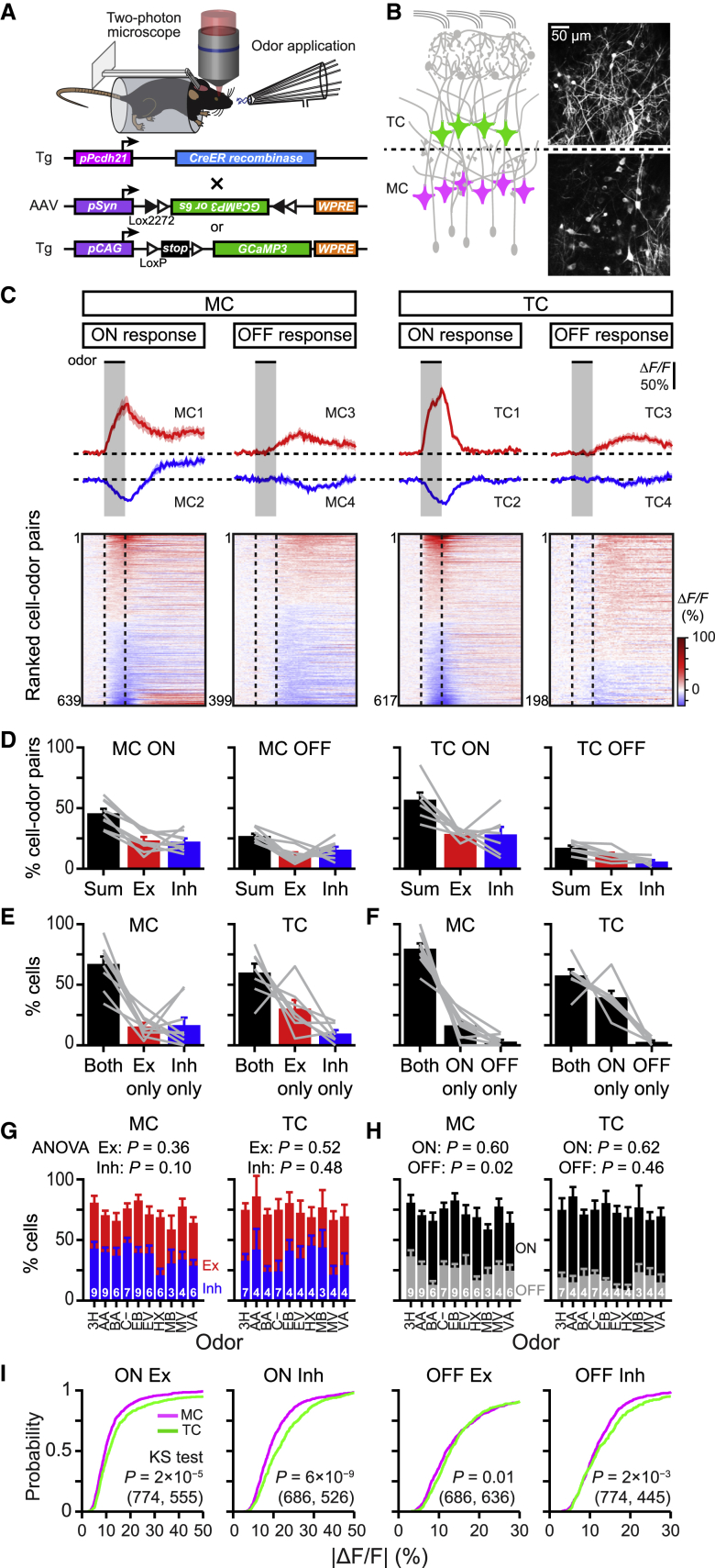
Comparable Odor-Evoked Response Profiles in MCs and TCs (A) Schema of the experimental paradigm. (B) Schema of the OB circuitry and example images of TCs (u223c120u00a0u03bcm deep; green) and MCs (u22...
Figureu00a02
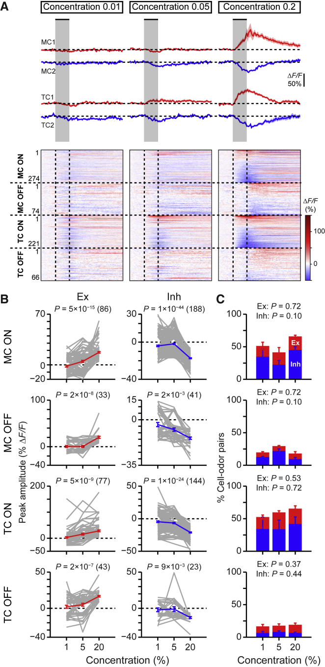
Concentration Dependency of Odor Responses in MC and TC Populations (A) Example traces and pseudo-color heatmaps (bottom) of statistically significant responses evoked by 2u00a0s odor application (bla...
Figureu00a03
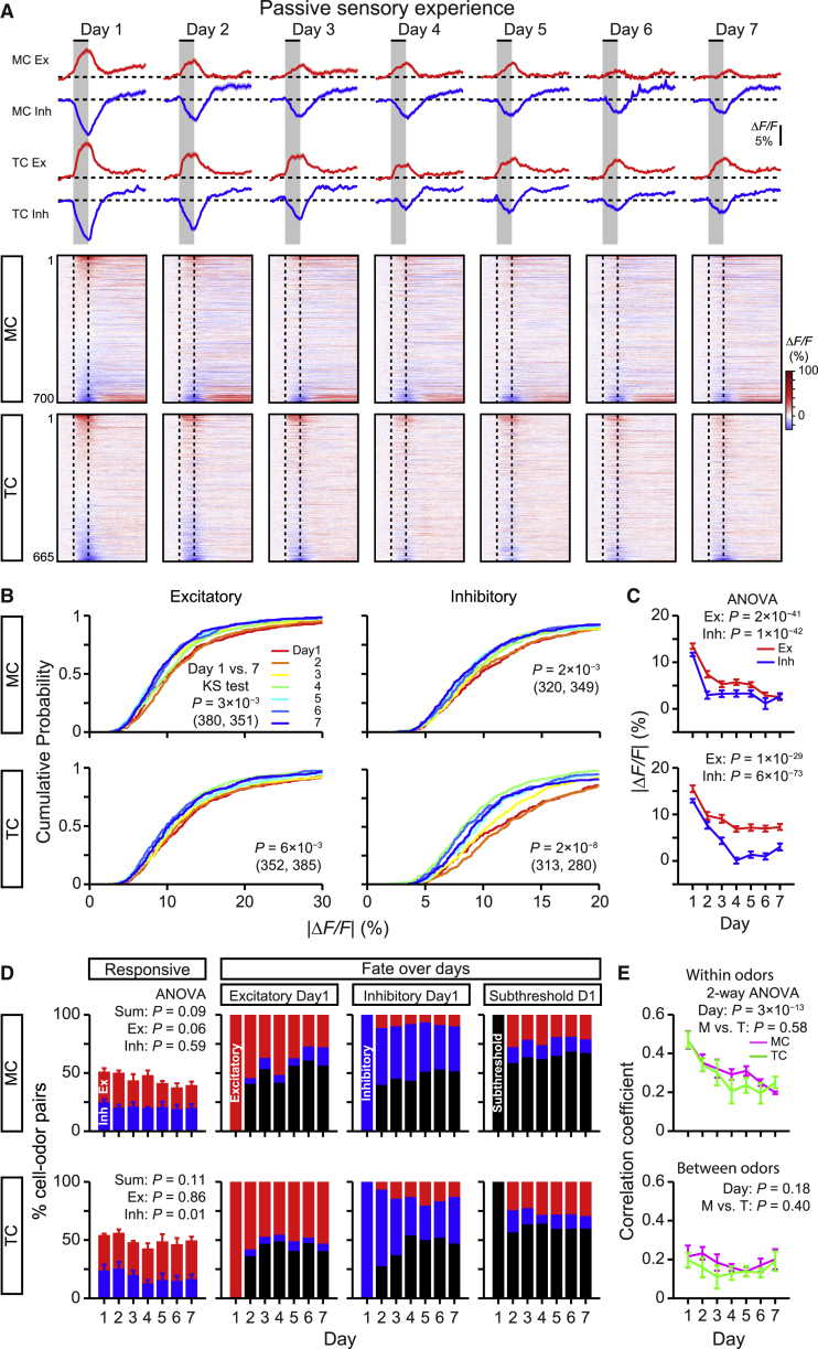
Similar Reorganization of Odor Representation in MCs and TCs after Passive Sensory Experience (A) Ca 2+ responses over 7u00a0days of passive sensory experience. Traces averaged across all cells based ...
Figureu00a04
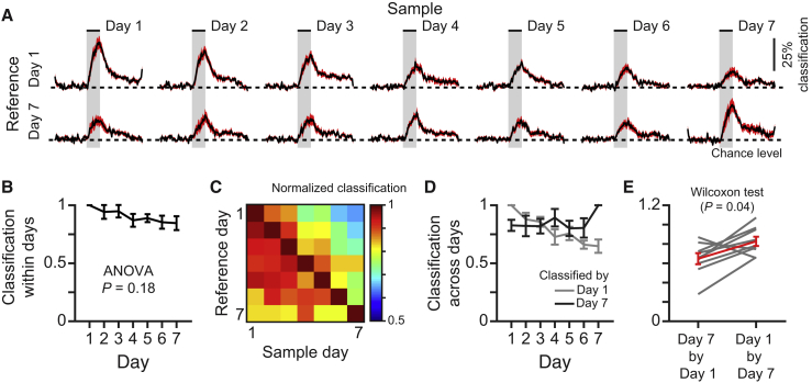
The Odor Representation Stabilizes after Passive Sensory Experience (A) Traces of percentage successful odor classification over time. Responses of sample days were classified by those of different re...
Figureu00a05
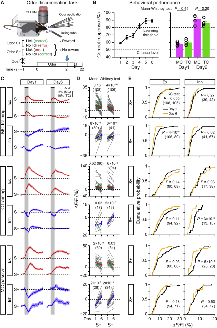
Changes of Odor Response Amplitudes in MCs and TCs after Active Sensory Learning (A) A schema of the odor discrimination task. Head-fixed mice were trained to discriminate between two binary mixtures ...
Figureu00a06
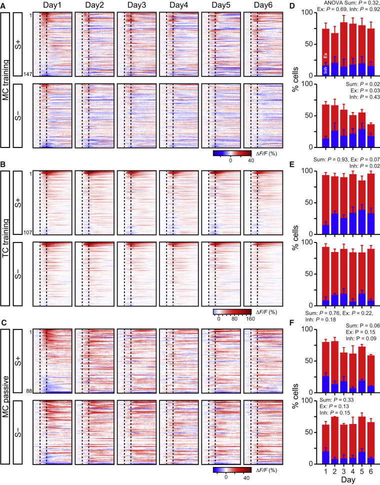
Changes of Ensemble Activity during Active Sensory Learning (Au2013C) Pseudo-color heatmaps of odor responses from all cells for MC training (A), TC training (B), and MC passive experience (C). Cell-o...
Figureu00a07
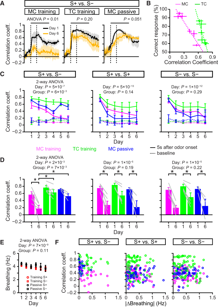
MC- and Active Learning-Specific Decrease of Ensemble Correlation (A) Traces of ensemble correlation between S+ and Su2212 responses. Population vectors of u0394F/F values from all cells were calculat...
Figureu00a08
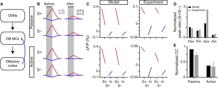
Cortical Feedback Can Account for the Context-Dependent Pattern Separation in MCs in a Computational Model (A) A schema representing our computational model. OSNs excite the OB projection neurons; the...
Figure images are served from the NIH/NLM PubMed Central Open Access Subset or Europe PMC; copyright remains with the publishers and authors.
💬 Discussion
0 commentsNo comments yet. Be the first to start a discussion!
Leave a Comment