Abstract
In vivo imaging at high spatiotemporal resolution is key to the understanding of complex biological systems. We integrated an optical phase-locked ultrasound lens into a two-photon fluorescence microscope and achieved microsecond-scale axial scanning, thus enabling volumetric imaging at tens of hertz. We applied this system to multicolor volumetric imaging of processes sensitive to motion artifacts, including calcium dynamics in behaving mouse brain and transient morphology changes and trafficking of immune cells.
🔬 Techniques
🧬 Organisms
💻 Software
✨ Fluorophores
🧪 Sample Preparation
🔬 Cell Lines
🏭 Microscope Brands
🧪 Reagent Suppliers
🔴 Lasers
📷 Detectors
🎨 Filters
💻 Software Details
💾 Data Repositories
🏛️ Research Organizations (ROR)
Affiliated research institutions:
📋 Methods
Setup
The key element is a precisely controlled ultrasound lens. To provide a reliable feedback of the lens oscillation, we combined a polarization-maintaining fiber coupled CW diode laser (LPS-PM785-FC, Thorlabs) and the fs laser (Chameleon, Coherent) with a dichroic mirror beam splitter (T810lpxr, Chroma). The CW laser beam went through the same path as the fs laser beam inside the OPLUL ( Supplementary Fig. 1a ). The ultrasound lens (TAG lens 2.0, TAG Optics) induced the laser beams to oscillate between converging and diverging states. We used a second dichroic mirror beam splitter to separate the CW beam from the fs beam and used an iris to spatially filter the CW beam. For converging beams, the optical power through the iris was higher. For diverging beams, the power was lower. By monitoring the beam intensity with the photodiode behind the iris, we precisely measured the ultrasound-induced lensing effect. To prevent the fs laser from entering the photodiode, we mounted a short-pass filter (FES0800, Thorlabs) on the photodiode. To maintain a consistent oscillation amplitude and phase, we employed a programmable digital PLL (HF2LI-PLL, Zurich Instruments) that used the photodiode signal as the feedback and drove the ultrasound transducer. Before locking the loop, we routinely measured the resonance peak ( Supplementary Fig. 1b ). We drove the lens near its ~455 kHz acoustic resonance peak and therefore a single axial scan took 1.1 microseconds (two axial scans per oscillation period). In this work, we only used the central area of the lens aperture (1.7 mm in diameter) whose refractive index profile was similar to that of a simple lens. As our galvo scanner had a 5 mm aperture, we used a 4f relay lens pair (AC254-100-B and AC253-300-B, Thorlabs) to magnify the laser beam by a factor of three. The objective lens used in all the imaging experiments was the Nikon 16x NA 0.8 water-dipping lens. The z scan range was ~40 microns. For applications requiring even longer axial range, we had a second configuration to achieve a ~130 microns range, in which we used a different relay lens pair (AC254-150-B and AC254-250-B, Thorlabs). In this configuration, the beam magnification was less and the beam did not completely fill the objective pupil. Therefore, we achieved a longer scan range at the cost of resolution. We inserted the OPLUL between the light source and the scanning microscope whose line rate ( x scan) was ~1 kHz. Therefore, we achieved a ~1 kHz frame rate in the x-z plane. Using a resonant galvo for the x scan, we can potentially achieve a frame rate of 10–30 kHz. The FPGA based DAQ system can simultaneously record and process data from three color channels: blue (filter ET460/36, Chroma); green (filter FF01-520/70, Semrock); red (filter FF01-625/90, Semrock).
Show full methods section
Setup
The key element is a precisely controlled ultrasound lens. To provide a reliable feedback of the lens oscillation, we combined a polarization-maintaining fiber coupled CW diode laser (LPS-PM785-FC, Thorlabs) and the fs laser (Chameleon, Coherent) with a dichroic mirror beam splitter (T810lpxr, Chroma). The CW laser beam went through the same path as the fs laser beam inside the OPLUL ( Supplementary Fig. 1a ). The ultrasound lens (TAG lens 2.0, TAG Optics) induced the laser beams to oscillate between converging and diverging states. We used a second dichroic mirror beam splitter to separate the CW beam from the fs beam and used an iris to spatially filter the CW beam. For converging beams, the optical power through the iris was higher. For diverging beams, the power was lower. By monitoring the beam intensity with the photodiode behind the iris, we precisely measured the ultrasound-induced lensing effect. To prevent the fs laser from entering the photodiode, we mounted a short-pass filter (FES0800, Thorlabs) on the photodiode. To maintain a consistent oscillation amplitude and phase, we employed a programmable digital PLL (HF2LI-PLL, Zurich Instruments) that used the photodiode signal as the feedback and drove the ultrasound transducer. Before locking the loop, we routinely measured the resonance peak ( Supplementary Fig. 1b ). We drove the lens near its ~455 kHz acoustic resonance peak and therefore a single axial scan took 1.1 microseconds (two axial scans per oscillation period). In this work, we only used the central area of the lens aperture (1.7 mm in diameter) whose refractive index profile was similar to that of a simple lens. As our galvo scanner had a 5 mm aperture, we used a 4f relay lens pair (AC254-100-B and AC253-300-B, Thorlabs) to magnify the laser beam by a factor of three. The objective lens used in all the imaging experiments was the Nikon 16x NA 0.8 water-dipping lens. The z scan range was ~40 microns. For applications requiring even longer axial range, we had a second configuration to achieve a ~130 microns range, in which we used a different relay lens pair (AC254-150-B and AC254-250-B, Thorlabs). In this configuration, the beam magnification was less and the beam did not completely fill the objective pupil. Therefore, we achieved a longer scan range at the cost of resolution. We inserted the OPLUL between the light source and the scanning microscope whose line rate ( x scan) was ~1 kHz. Therefore, we achieved a ~1 kHz frame rate in the x-z plane. Using a resonant galvo for the x scan, we can potentially achieve a frame rate of 10–30 kHz. The FPGA based DAQ system can simultaneously record and process data from three color channels: blue (filter ET460/36, Chroma); green (filter FF01-520/70, Semrock); red (filter FF01-625/90, Semrock).
Data acquisition and image reconstruction
As shown in the flow chart ( Supplementary Fig. 2 ), we used a high-speed data acquisition card to record both the PMT signals (from multiple channels of different colors) and the photodiode signal (optical feedback). As the required sampling rate was high, we used the fs laser’s pulse train as the external sample clock for the card. A high-speed comparator converted the analog pulse train signal into digital TTL pulses that were transmitted by a USB cable to the card. The start of each data recording was triggered by the laser scanning microscope’s line trigger. The photodiode signal contained the information of the axial scan position. We used a sinusoidal fitting of the photodiode signal to extract the phase and frequency of the axial scanning, from which we determined the exact axial position for every data point. We then applied a 2D linear interpolation to map the raw non-uniformly sampled x-z image onto a regularly spaced grid. The processed x-z frame contains 1024 × 40 voxels. We repeated the same procedure for different y positions and obtained the 3D image stack. For each channel, the sampling rate was 80 MHz and the effective voxel rate was 40 MHz. On average, two laser pulses contribute to the signal at one voxel. As an example, we show the raw data recorded for a 1 μm fluorescence bead ( Supplementary Fig. 3 ), from which we reconstructed the 3D volume images. All data shown is not averaged along the time axis unless otherwise specified. In the development stage, we used ScanImage to control the laser scanning microscope, and recorded data with a high-speed data acquisition card (ATS9440, AlazarTech). The recorded data was quickly streamed to data storage. We tested a RAM disk (DataRAM), internal SSD (840pro, SAMSUNG) and an external RAID system (CX3250, Colfax International); all provided sufficient throughput for the data streaming. The data processing (curve fitting and 2D interpolation) was done on a 2500-core cluster. Currently, we control the microscope by a custom Labview program and use a high-speed FPGA card (PXIe-7962R, NI) for data acquisition and processing in real time.
Code availability
The custom codes for hardware control and data analysis are available upon request from the authors. System calibration The OPLUL induced a slight degree of optical aberration. Using a recently demonstrated wavefront correction method 9 , we measured and compensated this system aberration ( Supplementary Fig. 4a, b ). After the aberration correction, we used 1 μm fluorescence beads embedded in 1.5% agarose to measure the axial scan range ( Supplementary Fig. 4c, d ). We used 0.2 μm fluorescence beads embedded in 1.5% agarose to measure the spatial resolution ( Supplementary Fig. 5 ). We further quantified the system performance over depth ( Supplementary Fig. 6 ) by in vivo deep imaging of fine structures, such as the dendrites and dendritic spines in S1 cortex of thy1-YFP (H line) transgenic mice. The spines can be resolved at up to ~400 μm depth (103 mW at 935 nm). Due to the ultrasound lens induced additional aberration, the axial resolution decreased when the focus was shifted away from the center. However, this did not substantially affect the resolution over the specified axial scanning ranges ( Supplementary Fig. 14 ). We compared the volume images recorded by the objective lens translation and by the OPLUL ( Supplementary Fig. 18 ), which shows the advantage of high-speed volume imaging in reducing the artifact caused by fast events. The signal-to-noise ratio (SNR) of each voxel depends on the excitation power, the brightness of the fluorophores, the imaging depth, the objective’s NA, the signal collection efficiency, the quantum efficiency of PMT, etc . We tested SNR with thy1-YFP (H line) transgenic mice in vivo and the typical single voxel SNR was ~5 in the fast volume imaging of fine structures such as the dendrites in the cortex (laser power ~ 100 mW at 935 nm, Nikon 16x NA 0.8 objective, PMT of ~50% quantum efficiency, imaging depth ~50–100 μm beneath the dura). With similar parameters, we also imaged the brains of CX3CR1 gfp/gfp transgenic mice; here the single voxel SNR was typically ~9.5 for fast volume imaging of microglial cell bodies (imaging depth ~100 μm). Considering that the power applied in our experiments is generally higher than that of 2D imaging, we performed photodamage quantification by 10 min continuous recording of calcium dynamics of deep somata and dendrites ( Supplementary Fig. 7 ). It is known that the photodamage is associated with an increase in basal fluorescence 21 . Despite the long time continuous imaging, the raw data ( Supplementary Fig. 7b, d ) shows no variation in the basal fluorescence of somata or small and dim structures such as dendrites.
Calcium imaging of mouse V1 neurons
All procedures involving mice were approved by the Animal Care and Use Committees of HHMI Janelia Research Campus and National Institute of Allergy and Infectious Diseases, National Institutes of Health. Mice approximately 6–12 weeks old of both sexes were used without randomization. The procedures related to the calcium imaging of C57BL/6 mouse V1 neurons with visual stimulation, including the V1 neuron labeling, the window surgery for acute experiments, the visual stimuli and the imaging of mouse V1 neurons, were conducted as in a previous report 22 with the following exceptions. (1) The visual stimuli were generated by a MATLAB program and displayed in blue color on a 7 inch LCD monitor. (2) Each stimulus trial included a 7 s blank period followed by a 4 s drifting sinusoidal grating. (3) The images were recorded at a higher speed. For the 2D cross-sectional calcium imaging of mouse V1 cortex ( Supplementary Fig. 8 ), the frame rate was 893 Hz with ~85 mW laser power (λ=935 nm). For the 3D calcium imaging of mouse visual cortex ( Supplementary Fig. 9 ), the volume was 375 × 375 × 130 μm 3 , and the volume rate was 5.6 Hz with ~100 mW laser power (λ=935 nm). Both the soma ensembles in the above results were at 100–250 μm beneath the dura. To monitor the spontaneous activity of V1 neurons, the mice were kept in the dark. During imaging, the mice were sedated with chlorprothixene (10–20 μL at 0.33 mg ml −1 , intramuscular), kept anesthetized (isoflurane, 0.5–2%), and were placed on a regulated heating pad (37 °C). For the volumetric imaging of dendritic segment in mouse V1 cortex ( Fig. 2a ), the volume size was 60 × 3.75 × 40 μm 3 and the volume rate was 56 Hz (85 mW at 935 nm). The imaging depth was 100–250 μm beneath the dura.
Calcium imaging in mouse S1 cortex
Surgeries were conducted on adult C57BL/6 mice under anesthesia (1.5–2% isoflurane). To reduce potential inflammation, 5 mg kg −1 ketofen was injected subcutaneously. 0.1 mg kg −1 buprenorphine was injected intraperitoneally to provide general analgesia. To label neurons of barrel cortex at layer 2/3, a small area craniotomy was performed over the left S1.
Virus expressing GCaMP6f
(AAV2/1-Syn-GCaMP6f) was injected slowly (30 nL in 5 mins) through the sharp tips of glass pipettes. After 1–2 weeks of expression, a craniotomy was performed above the former injection position, and a round imaging window made of two layers of microscope coverglass was mounted for chronic imaging experiments. Imaging was carried out 2–4 weeks after the craniotomy. Awake mice were placed on a regulated heating pad (37 °C) during the imaging. Puffs of compressed air (8 psi), with 500 ms duration and 5 s interval, were applied to the contralateral whiskers through a 1-mm-diameter tube placed ~15 mm away. The mice were tail-vein injected with Qtracker® 655 (blood plasma staining, Life Technologies) to label the blood vessels as references for motion registration. The laser power was ~60 mW at 935 nm. The imaging depth was 100–250 μm beneath the dura for the soma ensemble, and 0–100 μm beneath the dura for the dendrite network.
Calcium imaging in mouse M1 cortex
Surgeries were conducted on adult C57BL/6 mice under anesthesia (1.5–2% isoflurane). 5 mg kg −1 ketofen was injected subcutaneously to reduce potential inflammation, and 0.1 mg kg −1 buprenorphine was injected intraperitoneally to provide general analgesia. To label neurons of motor cortex at layer 2/3, a small area craniotomy was performed at 1.75 mm lateral and 0.13 mm rostal of bregma.
Virus expressing GCaMP6s
(AAV2/1-Syn-GCaMP6s) or the mixture of diluted AAV2/1-Syn-Cre and AAV2/1-Flex-Syn-GCaMP6f were injected slowly (30 nL in 5 mins) through the sharp tips of glass pipettes. After 1–2 weeks, the imaging window was installed above the former injection position after the craniotomy. The mice were trained to run on a linear treadmill after 1–2 weeks’ recovery. Imaging was carried out 2–4 weeks after the craniotomy. For the volumetric imaging of neuron ensemble in mouse M1 cortex ( Fig. 2g, h ), puffs of compressed air (6–8 psi), with 200 ms duration and 60 s interval, were applied to the contralateral whiskers (through a 1-mm-diameter tube placed ~15 mm away) of the head-restrained mice on a custom linear treadmill. The motion was monitored by an optical encoder mechanically coupled with the treadmill. The laser power was ~66 mW at 935 nm, and the imaging depth was 150–280 μm beneath the dura. For the photodamage quantification through calcium imaging of soma ensemble ( Supplementary Fig. 7a ), the head-restrained mice were running freely with no air puff applied. The laser power was ~125 mW at 935 nm, and the imaging depth was 370–500 μm beneath the dura. For the photodamage quantification through calcium imaging of neuron ensemble ( Supplementary Fig. 7c ), the head-restrained mice were kept standing in a plastic tube. The laser power was ~103 mW at 935 nm, and the imaging depth was 350–390 μm beneath the dura. Neutrophil imaging in mouse cerebral cortex and mouse ear To image neutrophils trafficking in mouse cerebral cortex, the Lyz2 gfp/+ B6.Albino mice 16 were first anesthetized (isoflurane, 1.5–2%), and a small area craniotomy was performed over the left S1. Astrocytes were stained by applying SR101 solution 23 for 2–3 mins before window installation. The mice were kept warm and anesthetized during the imaging. The laser power was ~90 mW (at 935 nm). The imaging of neutrophils in pial veins was performed at 0–60 μm beneath the dura, and the imaging of neutrophils in the capillaries of mouse cortex was performed at 50–150 μm beneath the dura. For neutrophil imaging in mouse ear, the Lyz2 gfp/+ B6.Albino mice were first anesthetized (isoflurane, 1.5–2%), and tail-vein injected with Qtracker® 655 to label the blood vessels. Another mouse strain, DsRed +/− Lyz2 gfp/+ B6.Albino mice 16 were used to visualize the blood vessel structure, without injecting blood tracer. Mild tissue damage was induced in the ear pinnae of the anesthetized mice before they were immobilized on a homemade stage. The mice were kept warm and anesthetized during the imaging. For the imaging of neutrophil trafficking in the ear vasculature of a Lyz2 gfp/+ B6.Albino transgenic mouse ( Supplementary Fig. 12 and Supplementary Video 17 ), the volume rate was 37 Hz (90 mW at 935 nm). For the 3D imaging of neutrophils rolling along the mouse ear vasculature of a Lyz2 gfp/+ B6.Albino transgenic mouse ( Supplementary Video 18 ), the volume rate was 19 Hz (100 mW at 935 nm). For the 3D imaging of neutrophils rolling along the mouse ear vasculature and extravascular tissue ( Supplementary Videos 19 and 20 ), the volume rate was 3.5 Hz (95 mW at 935 nm). The vascular systems in the above data sets were 50–250 μm beneath the mouse ear surface. Dendritic cell and lymphocyte cell imaging in mouse lymph nodes CD11c-EYFP 17 or Tbet:ZsGreen 18 transgenic mice (for dendritic cell and lymphocyte cell imaging, respectively), both from Taconic-NIH mouse exchange program, were anesthetized by continuous inhalation of isoflurane and immobilized on a homemade stage, after which the popliteal lymph node was carefully exposed surgically. During the imaging, the mice were kept warm by a temperature-regulated heating pad and under continuous anesthesia. The laser power was ~100 mW (at 935 nm). The motility and fluorescence of the labeled cells did not exhibit apparent alteration during the imaging that typically lasted a few minutes. The imaging depth was 10–250 μm beneath the surface of the popliteal lymph nodes.
Microglia imaging
Craniotomy was performed on the skull (2 mm posterior and 2 mm lateral to the Bregma point) of adult CX3CR1 gfp/gfp mice 20 under isoflurane anesthesia (1.5–2%). To image the microglia and astrocyte simultaneously, astrocyte was stained with SR101 solution for 2–3 mins before window installation. Then the mice were placed on a regulated heating pad (37 °C) and kept anesthetized while we monitored the dynamics of microglia. To visualize the blood flow, the mice were tail vein injected with Qtracker® 655 (Life Technologies) for blood plasma staining. To study the microglia’s response to neuron damage, R-GECO (Addgene) was injected 2~3 weeks before the craniotomy (same as the protocol of GCaMP6 virus injection, except for the injection position). The neuron was damaged via laser ablation 24 . The laser power for imaging microglia was ~100 mW at 935 nm. The microglia ensembles activated by BBB disruption ( Fig. 3f ) were 100–140 μm beneath the dura. The volumetric imaging of microglia and neuron ensembles ( Supplementary Videos 25–29 ) was 60–200 μm beneath the dura.
Image analysis
To correct motion artifacts, motion registrations were carried out with a cross correlation algorithm 25 . We manually chose the stacks with no apparent motion, and used the average intensity projections of these stacks along the time axis as the reference. Generally, we registered the MIPs of the volume (in x-y and x-z planes) at each time point with respect to MIPs of the reference, then aligned the volume accordingly. To define the region-of-interest in the imaging of dendrites and dendritic spines, we computed the standard deviation in time for every pixel in the volume. Reconstruction was performed in a semiautomated fashion using the Simple Neurite Tracer plugin in ImageJ. Reconstructions were manually inspected for accuracy. The three-dimensional masks for each spine and dendritic segment were generated after the reconstructions. We then computed the average Δ F/F in each mask-defined volume. To measure the neuronal activity of the soma ensemble, we performed MIP along the time axis of the 4D data after the image alignment. We detected and segmented the cells, as in the detection of mGRASP 26 . Each cell was segmented based on the seeded region growing method 27 . Using the cell’s mask, we were able to calculate the cell’s time domain response. We further processed the calcium dynamics of the neuron ensemble in M1 cortex using the following procedures. We performed meta-k-means clustering and Pearson’s correlation coefficient calculations (between any two calcium traces of interest), to identify the neurons of strong correlation with each other and with running (correlation coefficient > 0.7). Then we calculated the correlations of the mean activity trace of these neurons with that of each neuron, to distinguish the neurons with significant ( p < 0.05, t -test) positive correlation to running. We sorted the neurons first into their respective clusters and then within each cluster by their correlation to the cluster’s mean activity 28 ( Supplementary Fig. 10c ). For tracking the dendritic cells in lymph nodes, we selected a seed point for each cell of interest. Then we segmented the cell body around the seed point by means of the seeded region growing method 27 . We used Amira (FEI visualization sciences group) and Imaris (Bitplane) to prepare the figures and supplementary videos .
Supplementary Material 1
📊 Figures
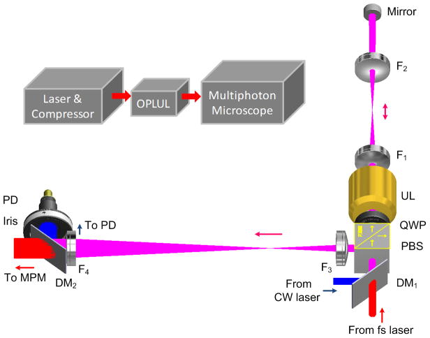
Figure 1
Design of the high-speed volumetric imaging system. A fs laser beam (two-photon excitation beam) and a CW diode laser beam (reference beam), both horizontally polarized, are combined by a dichroic mir...
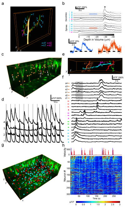
Figure 2
High-speed 3D in vivo calcium imaging of neuronal networks. ( a ) Representative volume view of a GCaMP6s-expressing dendritic segment (of 3 datasets) in mouse V1 cortex ( x u00d7 y u00d7 z : 60 u00d7...
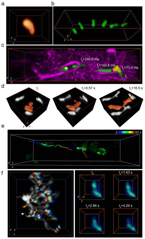
Figure 3
High-speed 3D in vivo imaging of cell dynamics. ( a ) A representative neutrophil image reconstructed from 2D cross sectional imaging of a pial vein in mouse brain at 1 kHz frame rate at depth 5u20134...
Figure images are served from the NIH/NLM PubMed Central Open Access Subset or Europe PMC; copyright remains with the publishers and authors.
💬 Discussion
0 commentsNo comments yet. Be the first to start a discussion!
Leave a Comment