Abstract
Chromatin conformation regulates gene expression and thus, constant remodeling of chromatin structure is essential to guarantee proper cell function. To gain insight into the spatiotemporal organization of the genome, we use high-density photoactivated localization microscopy and deep learning to obtain temporally resolved super-resolution images of chromatin in living cells. In combination with high-resolution dense motion reconstruction, we find elongated ~45- to 90-nm-wide chromatin "blobs." A computational chromatin model suggests that these blobs are dynamically associating chromatin fragments in close physical and genomic proximity and adopt topologically associated domain-like interactions in the time-average limit. Experimentally, we found that chromatin exhibits a spatiotemporal correlation over ~4 μm in space and tens of seconds in time, while chromatin dynamics are correlated over ~6 μm and last 40 s. Notably, chromatin structure and dynamics are closely related, which may constitute a mechanism to grant access to regions with high local chromatin concentration.
🔬 Techniques
🔭 Microscopes
💻 Software
✨ Fluorophores
🧪 Sample Preparation
🔬 Cell Lines
🏭 Microscope Brands
🧪 Reagent Suppliers
📷 Detectors
🎨 Filters
💻 Software Details
💻 Code & Software
💾 Data Repositories
🏛️ Research Organizations (ROR)
Affiliated research institutions:
📋 Methods
Cell culture Human osteosarcoma U2OS expressing
H2B-PATagRFP cells were a gift from S. Huet (CNRS, UMR 6290, Institut Génétique et Développement de Rennes, Rennes, France); the histone H2B was cloned, as described previously ( 34 ). U2OS cells were cultured in Dulbecco’s modified Eagle’s medium [with glucose (4.5 g/liter)] supplemented with 10% fetal bovine serum (FBS), 2 mM glutamine, penicillin (100 μg/ml), and streptomycin (100 U/ml) in 5% CO 2 at 37°C. Cells were plated 24 hours before imaging on 35-mm petri dishes with a no. 1.5 coverslip-like bottom (ibidi, Biovalley) with a density of 2 × 10 5 cells per dish. Just before imaging, the growth medium was replaced by Leibovitz’s L-15 medium (Life Technologies) supplemented with 20% FBS, 2 mM glutamine, penicillin (100 μg/ml), and streptomycin (100 U/ml).
PALM imaging in living cells
Imaging of H2B-PAtagRFP in living
U2OS cells was carried out on a fully automated Nikon Ti-E/B PALM (Nikon Instruments) microscope. The microscope is equipped with a full incubator enclosure with gas regulation to maintain a temperature of ~37°C for normal cell growth during live-cell imaging. Image sequences of 2000 frames were recorded with an exposure time of 30 ms per frame (33.3 frames/s). For Deep-PALM imaging, a relatively low power (~50 W/cm 2 at the sample) was applied for H2B-PATagRFP excitation at 561 nm and then combined with the 405 nm (~2 W/cm 2 at the sample) to photoactivate the molecules between the states. Note that for Deep-PALM imaging, switched fluorophores are not required to stay as long in the dark state as for conventional PALM imaging. We used oblique illumination microscopy ( 11 ) combined with total internal reflection fluorescence (TIRF) mode to illuminate a thin layer of 200 nm (axial resolution) across the nucleus. The reconstruction of super-resolved images improves the axial resolution only marginally (fig. S1, E and F). Laser beam powers were controlled by acoustic optic-modulators (AA Opto-Electronic). Both wavelengths were united into an oil immersion 1.49-NA (numerical aperture) TIRF objective (100×; Nikon). An oblique illumination was applied to acquire image series with a high signal-to-noise ratio. The fluorescence emission signal was collected by using the same objective and spectrally filtered by a Quad-Band beam splitter (ZT405/488/561/647rpc-UF2, Chroma Technology) with a Quad-Band emission filter (ZET405/488/561/647m-TRF, Chroma Technology). The signal was recorded on an electron-multiplying charge-coupled device camera (Andor iXon X3 DU-897, Andor Technology) with a pixel size of 108 nm. For axial correction, Perfect Focus System was applied to correct for defocusing. NIS-Elements software was used for acquiring the images. PALM imaging and PALM data analysis in fixed cells The same cell line (U2OS expressing H2B-PAtagRFP), as in live-cell imaging, was used for conventional PALM imaging. Before fixation, cells were washed with phosphate-buffered saline (PBS) (three times for 5 min each) and then fixed with 4% paraformaldehyde (Sigma-Aldrich) diluted in PBS for 15 min at room temperature. A movie of 8000 frames was acquired with an exposure time of 30 ms per frame (33.3 frames/s). In comparison to Deep-PALM imaging, a relatively higher excitation laser of 561 nm (~60 W/cm 2 at the sample) was applied to photobleach H2B-PATagRFP and then combined with the 405 nm (~2.5 W/cm 2 at the sample) for photoactivating the molecules. We used the same oblique illumination microscopy combined with TIRF system, as applied in live-cell imaging. PALM images from fixed cells were analyzed using ThunderSTORM ( 35 ). Super-resolution images were constructed by binning emitter localizations into 13.5 × 13.5 nm pixels and blurred by a Gaussian to match Deep-PALM images. The image segmentation was carried out as on images from living cells (see below). Deep-PALM analysis The CNN was trained using simulated data following Nehme et al . ( 15 ) for three labeling densities (4, 6, and 9 emitters/μm 2 per frame). Raw imaging data were checked for drift, as previously described ( 12 ). The detected drift in raw images is in the range of 0.99 I max ; fig. S3B). Since blobs are characterized by surrounding pixels of considerably less density, the Euclidian distance transform is computed on the binary foreground markers. Background pixels (i.e., those pixels not belonging to any blobs) are expected to lie far away from any blob center, and thus, a good estimate for background markers are those pixels being furthest from any foreground pixel. We hence compute the watershed transform on the distance transform of foreground markers, and the resulting watershed lines depict background pixels (fig. S3C). Equipped with fore- and background markers (fig. S3D), we apply a marker-controlled watershed transform on the gradient of the input image (fig. S3E). The marker-controlled watershed imposes minima on marker pixels, preventing the formation of watershed lines across marker pixels. Therefore, the marker-controlled watershed accurately detects boundaries and blobs that might not have been previously marked as foreground (fig. S3F). Last, spurious blobs whose median- or mean intensity is below 10% of the maximum intensity are discarded, and each blob is assigned a unique label for further correspondence (fig. S3G). The area and centroid position are computed for each identified blob for further analysis. This automated segmentation scheme performs considerably better than other state-of-the-art algorithms for image segmentation because of the reliable identification of fore- and background markers accompanied by the watershed transform (note S1). Chromatin blob properties Centroid position, area, and eccentricity were computed. The eccentricity is computed by describing the blobs as an ellipse E = 1 − a 2 / b 2 (3) where a and b are the short and long axes of the ellipse, respectively. Chromatin blob identification from a computational chromatin model We chose to use a computational chromatin model, recently introduced by Qi and Zhang ( 19 ), to elucidate the origin of experimentally determined chromatin blobs. Each bead of the model covers a sequence length of 5 kb and is assigned 1 of 15 chromatin states to distinguish promoters, enhancers, quiescent chromatin, etc. Starting from the simulated polymer configurations, we consider monomers within a 200-nm-thick slab through the center of the simulated chromosome. To generate super-resolved images as those from Deep-PALM analysis, fluorescence intensity is ascribed to each monomer. Monomer positions are subsequently discretized on a grid with 13.5-nm spacing and convolved with a narrow point-spread function, which results in images closely resembling experimental Deep-PALM images of chromatin. Chromatin blobs were then be identified and characterized as on experimental data ( Fig. 2, A and B ). Mapping back the association of each bead to a blob (if any) allows us to analyze principles of blob formation and maintenance using the distance and the association strength between each pair of monomers, averaged over all 20,000 simulated polymer configurations. Radial distribution function The radial distribution function g ( r ) (also pair correlation function) is calculated (in two dimensions) by counting the number of blobs in an annulus of radius r and thickness dr . The result is normalized by the bulk density ρ = n / A , with the total number of blobs n and, A , the area of the nucleus, and the area of the annulus, 2π r dr dn ( r ) = ρ · g ( r ) · 2 π r dr (4) Quantification of chromatin dynamics Super-resolved images of chromatin showed spatially distributed blobs of varying size, but the resolved structure is too dense for state-of-the-art single-particle tracking methods to track. Furthermore are highly dynamic structures, assembling and dissembling within one to two super-resolved frames ( Fig. 3D ), which makes a single-particle tracking approach unsuitable. Instead, we used a method for dynamics reconstruction of bulk macromolecules with dense labeling, optical flow. Optical flow builds on the computation of flow fields between two successive frames of an image series. The integration of these flow fields from super-resolution images results in trajectories displaying the local motion of bulk chromatin with temporal and high spatial resolution. Further, the trajectories are classified into various diffusion models, and parameters describing the underlying motion are computed ( 14 ). Here, we use the effective diffusion coefficient D (in units of m 2 /s α ), which reflects the magnitude of displacements between successive frames (the velocity of particles or monomers in the continuous limit) and the anomalous exponent α ( 14 ). The anomalous exponent reflects whether the diffusion is free (α = 1, e.g., for noninteracting particles in solution), directed (α > 1, e.g., as the result from active processes), or hindered (α < 1, e.g., because of obstacles or an effective back-driving force). Furthermore, we compute the length of constraint L c , which is defined as the SD of the trajectory positions with respect to its time-averaged position. Denoting R ( t ; R 0 ), the trajectory at time t originating from R 0 , the expression reads L c ( R 0 ) = var( R ( t ; R 0 )) 1/2 , where var denotes the variance. The length of constraint is a measure of the length scale explored of the monomer during the observation period. A complementary measure is the confinement level ( 39 ), which computes the inverse of the variance of displacements within a sliding window of length ω: C ∝ ω/ var( R ( t ; R 0 )), where the sliding window length is set to four frames (1.44 s). Larger values of C denote a more confined state than small ones. Spatial correlation for temporally varying parameters The NND and the area, as well as the flow magnitude, were calculated and assigned to the blobs’ centroid position. To calculate the spatial correlation between parameters, the parameters were interpolated from the scattered centroid positions onto a regular grid spanning the entire nucleus. Because not every pixel in the original super-resolved images is assigned a parameter value, we chose an effective grid spacing of five pixels (67.5 nm) for the interpolated parameter maps. After interpolation, the spatial correlation was computed between parameter pairs: Let r = ( x , y ) T denote a position on a regular two-dimensional grid and f ( r , t ) and g ( r , t ) two scalar fields with mean zero and variance one, at time t on that grid. The time series of parameter fields consist of N time points. The spatial cross-correlation between the fields f and g , which lie a lag time τ apart, is then calculated as C ( ρ , τ ) = 1 N ∑ t ∑ x , y f ( r , t ) g ( r + ρ , t + τ ) ∑ x , y f ( r , t ) g ( r , t + τ ) (5) where the space lag ρ is a two-dimensional vector ρ = (Δ x , Δ y ) T . The sums in the numerator and denominator are taken over the spatial dimensions; the first sum is taken over time. The average is thus taken over all time points that are compliant with time lag τ. Subsequently, the radial average in space is taken over the correlation, thus effectively calculating the spatial correlation C (ρ, τ) over the space lag ρ = Δ x 2 + Δ y 2 . If f = g , then the spatial autocorrelation is computed.
Show full methods section
Cell culture Human osteosarcoma U2OS expressing
H2B-PATagRFP cells were a gift from S. Huet (CNRS, UMR 6290, Institut Génétique et Développement de Rennes, Rennes, France); the histone H2B was cloned, as described previously ( 34 ). U2OS cells were cultured in Dulbecco’s modified Eagle’s medium [with glucose (4.5 g/liter)] supplemented with 10% fetal bovine serum (FBS), 2 mM glutamine, penicillin (100 μg/ml), and streptomycin (100 U/ml) in 5% CO 2 at 37°C. Cells were plated 24 hours before imaging on 35-mm petri dishes with a no. 1.5 coverslip-like bottom (ibidi, Biovalley) with a density of 2 × 10 5 cells per dish. Just before imaging, the growth medium was replaced by Leibovitz’s L-15 medium (Life Technologies) supplemented with 20% FBS, 2 mM glutamine, penicillin (100 μg/ml), and streptomycin (100 U/ml).
PALM imaging in living cells
Imaging of H2B-PAtagRFP in living
U2OS cells was carried out on a fully automated Nikon Ti-E/B PALM (Nikon Instruments) microscope. The microscope is equipped with a full incubator enclosure with gas regulation to maintain a temperature of ~37°C for normal cell growth during live-cell imaging. Image sequences of 2000 frames were recorded with an exposure time of 30 ms per frame (33.3 frames/s). For Deep-PALM imaging, a relatively low power (~50 W/cm 2 at the sample) was applied for H2B-PATagRFP excitation at 561 nm and then combined with the 405 nm (~2 W/cm 2 at the sample) to photoactivate the molecules between the states. Note that for Deep-PALM imaging, switched fluorophores are not required to stay as long in the dark state as for conventional PALM imaging. We used oblique illumination microscopy ( 11 ) combined with total internal reflection fluorescence (TIRF) mode to illuminate a thin layer of 200 nm (axial resolution) across the nucleus. The reconstruction of super-resolved images improves the axial resolution only marginally (fig. S1, E and F). Laser beam powers were controlled by acoustic optic-modulators (AA Opto-Electronic). Both wavelengths were united into an oil immersion 1.49-NA (numerical aperture) TIRF objective (100×; Nikon). An oblique illumination was applied to acquire image series with a high signal-to-noise ratio. The fluorescence emission signal was collected by using the same objective and spectrally filtered by a Quad-Band beam splitter (ZT405/488/561/647rpc-UF2, Chroma Technology) with a Quad-Band emission filter (ZET405/488/561/647m-TRF, Chroma Technology). The signal was recorded on an electron-multiplying charge-coupled device camera (Andor iXon X3 DU-897, Andor Technology) with a pixel size of 108 nm. For axial correction, Perfect Focus System was applied to correct for defocusing. NIS-Elements software was used for acquiring the images. PALM imaging and PALM data analysis in fixed cells The same cell line (U2OS expressing H2B-PAtagRFP), as in live-cell imaging, was used for conventional PALM imaging. Before fixation, cells were washed with phosphate-buffered saline (PBS) (three times for 5 min each) and then fixed with 4% paraformaldehyde (Sigma-Aldrich) diluted in PBS for 15 min at room temperature. A movie of 8000 frames was acquired with an exposure time of 30 ms per frame (33.3 frames/s). In comparison to Deep-PALM imaging, a relatively higher excitation laser of 561 nm (~60 W/cm 2 at the sample) was applied to photobleach H2B-PATagRFP and then combined with the 405 nm (~2.5 W/cm 2 at the sample) for photoactivating the molecules. We used the same oblique illumination microscopy combined with TIRF system, as applied in live-cell imaging. PALM images from fixed cells were analyzed using ThunderSTORM ( 35 ). Super-resolution images were constructed by binning emitter localizations into 13.5 × 13.5 nm pixels and blurred by a Gaussian to match Deep-PALM images. The image segmentation was carried out as on images from living cells (see below). Deep-PALM analysis The CNN was trained using simulated data following Nehme et al . ( 15 ) for three labeling densities (4, 6, and 9 emitters/μm 2 per frame). Raw imaging data were checked for drift, as previously described ( 12 ). The detected drift in raw images is in the range of 0.99 I max ; fig. S3B). Since blobs are characterized by surrounding pixels of considerably less density, the Euclidian distance transform is computed on the binary foreground markers. Background pixels (i.e., those pixels not belonging to any blobs) are expected to lie far away from any blob center, and thus, a good estimate for background markers are those pixels being furthest from any foreground pixel. We hence compute the watershed transform on the distance transform of foreground markers, and the resulting watershed lines depict background pixels (fig. S3C). Equipped with fore- and background markers (fig. S3D), we apply a marker-controlled watershed transform on the gradient of the input image (fig. S3E). The marker-controlled watershed imposes minima on marker pixels, preventing the formation of watershed lines across marker pixels. Therefore, the marker-controlled watershed accurately detects boundaries and blobs that might not have been previously marked as foreground (fig. S3F). Last, spurious blobs whose median- or mean intensity is below 10% of the maximum intensity are discarded, and each blob is assigned a unique label for further correspondence (fig. S3G). The area and centroid position are computed for each identified blob for further analysis. This automated segmentation scheme performs considerably better than other state-of-the-art algorithms for image segmentation because of the reliable identification of fore- and background markers accompanied by the watershed transform (note S1). Chromatin blob properties Centroid position, area, and eccentricity were computed. The eccentricity is computed by describing the blobs as an ellipse E = 1 − a 2 / b 2 (3) where a and b are the short and long axes of the ellipse, respectively. Chromatin blob identification from a computational chromatin model We chose to use a computational chromatin model, recently introduced by Qi and Zhang ( 19 ), to elucidate the origin of experimentally determined chromatin blobs. Each bead of the model covers a sequence length of 5 kb and is assigned 1 of 15 chromatin states to distinguish promoters, enhancers, quiescent chromatin, etc. Starting from the simulated polymer configurations, we consider monomers within a 200-nm-thick slab through the center of the simulated chromosome. To generate super-resolved images as those from Deep-PALM analysis, fluorescence intensity is ascribed to each monomer. Monomer positions are subsequently discretized on a grid with 13.5-nm spacing and convolved with a narrow point-spread function, which results in images closely resembling experimental Deep-PALM images of chromatin. Chromatin blobs were then be identified and characterized as on experimental data ( Fig. 2, A and B ). Mapping back the association of each bead to a blob (if any) allows us to analyze principles of blob formation and maintenance using the distance and the association strength between each pair of monomers, averaged over all 20,000 simulated polymer configurations. Radial distribution function The radial distribution function g ( r ) (also pair correlation function) is calculated (in two dimensions) by counting the number of blobs in an annulus of radius r and thickness dr . The result is normalized by the bulk density ρ = n / A , with the total number of blobs n and, A , the area of the nucleus, and the area of the annulus, 2π r dr dn ( r ) = ρ · g ( r ) · 2 π r dr (4) Quantification of chromatin dynamics Super-resolved images of chromatin showed spatially distributed blobs of varying size, but the resolved structure is too dense for state-of-the-art single-particle tracking methods to track. Furthermore are highly dynamic structures, assembling and dissembling within one to two super-resolved frames ( Fig. 3D ), which makes a single-particle tracking approach unsuitable. Instead, we used a method for dynamics reconstruction of bulk macromolecules with dense labeling, optical flow. Optical flow builds on the computation of flow fields between two successive frames of an image series. The integration of these flow fields from super-resolution images results in trajectories displaying the local motion of bulk chromatin with temporal and high spatial resolution. Further, the trajectories are classified into various diffusion models, and parameters describing the underlying motion are computed ( 14 ). Here, we use the effective diffusion coefficient D (in units of m 2 /s α ), which reflects the magnitude of displacements between successive frames (the velocity of particles or monomers in the continuous limit) and the anomalous exponent α ( 14 ). The anomalous exponent reflects whether the diffusion is free (α = 1, e.g., for noninteracting particles in solution), directed (α > 1, e.g., as the result from active processes), or hindered (α < 1, e.g., because of obstacles or an effective back-driving force). Furthermore, we compute the length of constraint L c , which is defined as the SD of the trajectory positions with respect to its time-averaged position. Denoting R ( t ; R 0 ), the trajectory at time t originating from R 0 , the expression reads L c ( R 0 ) = var( R ( t ; R 0 )) 1/2 , where var denotes the variance. The length of constraint is a measure of the length scale explored of the monomer during the observation period. A complementary measure is the confinement level ( 39 ), which computes the inverse of the variance of displacements within a sliding window of length ω: C ∝ ω/ var( R ( t ; R 0 )), where the sliding window length is set to four frames (1.44 s). Larger values of C denote a more confined state than small ones. Spatial correlation for temporally varying parameters The NND and the area, as well as the flow magnitude, were calculated and assigned to the blobs’ centroid position. To calculate the spatial correlation between parameters, the parameters were interpolated from the scattered centroid positions onto a regular grid spanning the entire nucleus. Because not every pixel in the original super-resolved images is assigned a parameter value, we chose an effective grid spacing of five pixels (67.5 nm) for the interpolated parameter maps. After interpolation, the spatial correlation was computed between parameter pairs: Let r = ( x , y ) T denote a position on a regular two-dimensional grid and f ( r , t ) and g ( r , t ) two scalar fields with mean zero and variance one, at time t on that grid. The time series of parameter fields consist of N time points. The spatial cross-correlation between the fields f and g , which lie a lag time τ apart, is then calculated as C ( ρ , τ ) = 1 N ∑ t ∑ x , y f ( r , t ) g ( r + ρ , t + τ ) ∑ x , y f ( r , t ) g ( r , t + τ ) (5) where the space lag ρ is a two-dimensional vector ρ = (Δ x , Δ y ) T . The sums in the numerator and denominator are taken over the spatial dimensions; the first sum is taken over time. The average is thus taken over all time points that are compliant with time lag τ. Subsequently, the radial average in space is taken over the correlation, thus effectively calculating the spatial correlation C (ρ, τ) over the space lag ρ = Δ x 2 + Δ y 2 . If f = g , then the spatial autocorrelation is computed.
Spatial correlation for static parameters
We denote as global parameters those that reflect the structural and dynamic behavior of chromatin spatially resolved in a time-averaged manner. Examples involve the diffusion constant, the anomalous exponent, the length of constraint, but also time-averaged NND maps, etc. (fig. S8). Those parameters are useful to determine time-universal characteristics. The spatial correlation between those parameters is equivalent to the expression given for temporally varying parameters when the temporal dimension is omitted, effectively resulting in a correlation curve C (ρ). t-distributed stochastic neighbor embedding The distance from the periphery, intensity, their NND, area, flow magnitude, and confinement level of each identified blob form the six-dimensional–input feature space for t -SNE analysis. The parameters for each blob ( n = 3,260,232; divided into subsets of approximately 10,000) were z -transformed before the t -SNE analysis. The t -SNE analysis was performed using MATLAB and the Statistics and Machine Learning Toolbox (Release 2017b; The MathWorks Inc., Natick, MA, USA) with the Barnes-Hut approximation. The algorithm was tested using different distance metrics and perplexity values and showed robust results within the examined ranges (note S3 and fig. S10).
Supplementary Material aaz2196_SM.pdf aaz2196_Movie_S1.avi
📊 Figures
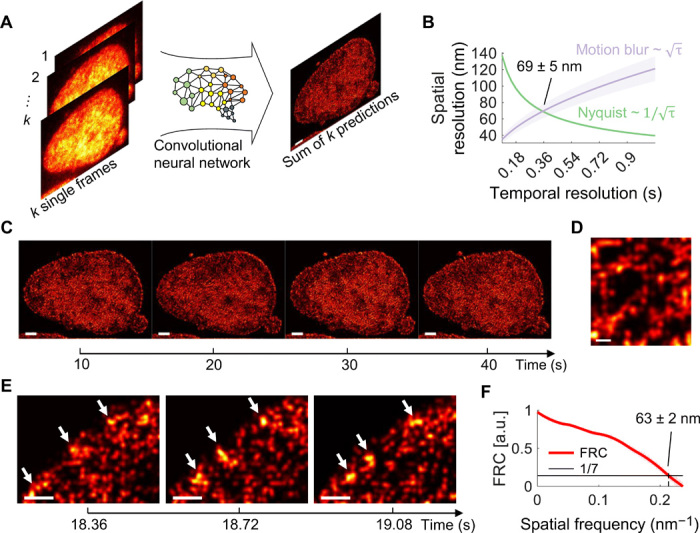
Fig. 1
Temporally resolved super-resolution images of chromatin in U2OS nuclei.
( A ) Wide-field images of U2OS nuclei expressing H2B-PATagRFP are input to a trained CNN, and predictions from multiple input frames are summed to construct a super-resolved image of chromatin in viv...
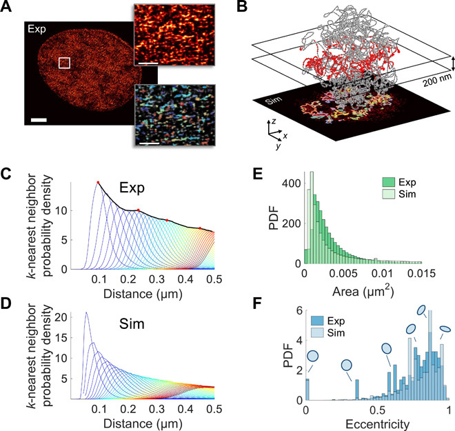
Fig. 2
Chromatin blob identification and characterization of imaged and modeled chromatin.
( A ) Super-resolved images show blobs of chromatin (left). These blobs are segmented (see Materials and Methods and note S1) and individually labeled by random color (right). Magnifications of the bo...
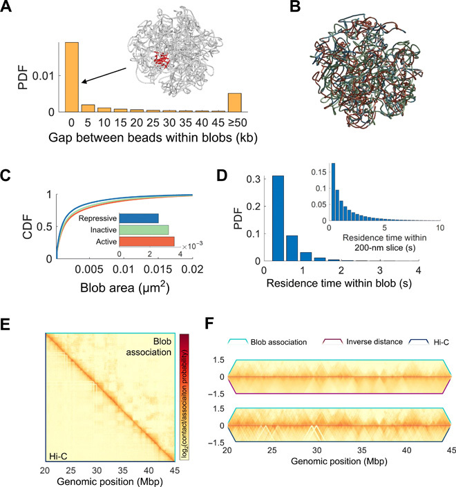
Fig. 3
Chromatin blobs on modeled chromosomes consist of continuous loci along the genome and exhibit a TAD-like time-averaged conformation.
( A ) Gap length between beads belonging to the same blob. An exemplary blob with small gap length is shown. The blob is mostly made of consecutive beads being in close spatial proximity. ( B ) A repr...
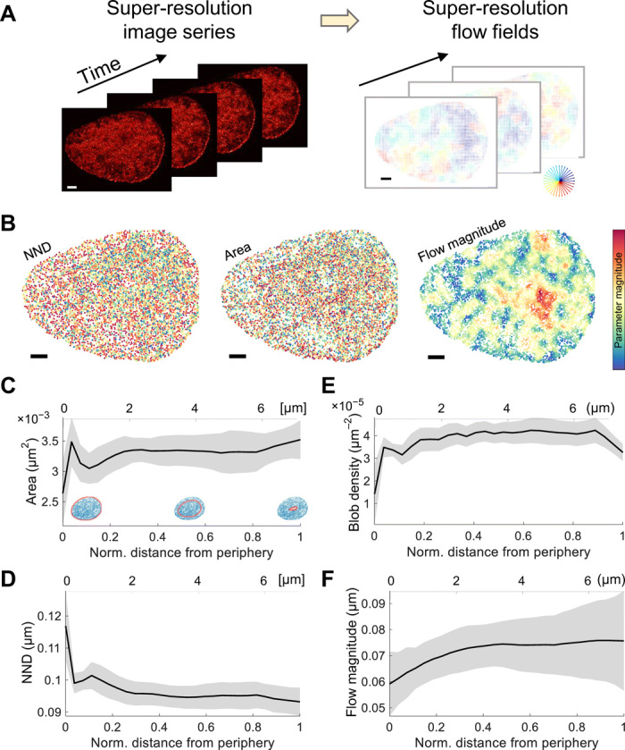
Fig. 4
Structural and dynamics blob characteristics dependent on the proximity to the nuclear periphery.
( A ) A time series of super-resolution images (left) is subject to optical flow (right). ( B ) Blobs of a representative nucleus (see movie S1) are labeled by their NND (left), area (middle), and flo...
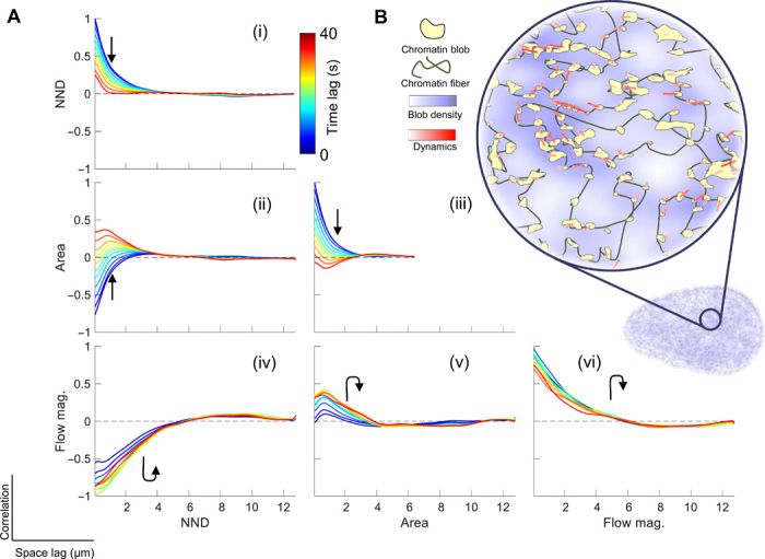
Fig. 5
Spatiotemporal correlations between structural and dynamic parameters.
( A ) The spatial auto- and cross-correlation between parameters were computed for different time lags. The graphs depict the correlation over space lag for each parameter pair, and different colors d...
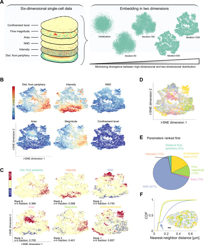
Fig. 6
Chromatin feature extraction.
( A ) The six-dimensional parameter space is input to the t -SNE algorithm and projected to two dimensions. ( B ) The two-dimensional embedding of an exemplary dataset is shown and colored according t...
Figure images are served from the NIH/NLM PubMed Central Open Access Subset or Europe PMC; copyright remains with the publishers and authors.
💬 Discussion
0 commentsNo comments yet. Be the first to start a discussion!
Leave a Comment