Abstract
One goal of cell biology is to understand how cells adopt different shapes in response to varying environmental and cellular conditions. Achieving a comprehensive understanding of the relationship between cell shape and environment requires a systems-level understanding of the signalling networks that respond to external cues and regulate the cytoskeleton. Classical biochemical and genetic approaches have identified thousands of individual components that contribute to cell shape, but it remains difficult to predict how cell shape is generated by the activity of these components using bottom-up approaches because of the complex nature of their interactions in space and time. Here, we describe the regulation of cellular shape by signalling systems using a top-down approach. We first exploit the shape diversity generated by systematic RNAi screening and comprehensively define the shape space a migratory cell explores. We suggest a simple Boolean model involving the activation of Rac and Rho GTPases in two compartments to explain the basis for all cell shapes in the dataset. Critically, we also generate a probabilistic graphical model to show how cells explore this space in a deterministic, rather than a stochastic, fashion. We validate the predictions made by our model using live-cell imaging. Our work explains how cross-talk between Rho and Rac can generate different cell shapes, and thus morphological heterogeneity, in genetically identical populations.
🔬 Techniques
🧬 Organisms
✨ Fluorophores
🧪 Sample Preparation
🏭 Microscope Brands
🧪 Reagent Suppliers
🏛️ Research Organizations (ROR)
Affiliated research institutions:
📋 Methods
5.1.
Software
Analyses were performed using M atlab . 5.2.
Dataset
The dataset used in this study was generated in an image-based screen of 256 TCs, where genes were either systematically inhibited by RNAi or overexpressed by transient transfection. In a limited number of TCs, there is a combination of overexpression and RNAi [ 26 ]. Cells were stochastically labelled with EGFP to facilitate image segmentation. For all TCs, 145 features were measured for 12 061 cells. 5.3.
Data transformation and reduction
All measured features are scaled between 0 and 1. After scaling, a constant of 0.01 is added to all measurements to make them non-zero and then a logarithmic transformation is applied. PCA is performed on the transformed data. The first three PCs analysed represent 59% of the variability in the original data and are considered for further analysis. Each other PC represented less than 5% of the variability in the original data and thus all have been discarded. Eigenvalues for this analysis are listed in the electronic supplementary material, tables S1 and S2. 5.4.
Single-cell clustering
For both hierarchical clustering and Gaussian mixture models, clusters are computed by varying the number of clusters ( k ) between five and 30. Hierarchical clustering is performed with Euclidean distance and Ward linkage. Gaussian mixture modelling is performed 10 times for each k and the final clustering with the best log-likelihood value is chosen. The average of silhouette values is used to assess the quality of the computed models, and the model with the highest average silhouette score is chosen. 5.5. Clustering performance improvement The chosen model has an average silhouette value of 0.7647. To improve the clustering performance, we divide the cells into two groups: cells with high silhouette values (more than 0.6) and cells with low silhouette values (less than 0.6). Next, we reclassify cells in the second group to those in the first group using KNN search, where k = 10. The final model achieves an average silhouette value of 0.7758. 5.6. Treatment condition heterogeneity profiles For each TC, including the wild-type (cells expressing EGFP alone) population, the percentage of cells in each shape is computed, resulting in a vector describing the distribution of cells for each TC. These vectors are then normalized by subtracting the wild-type TCHP. All THCPs are listed in the electronic supplementary material, table S3. 5.7. Normalized treatment condition heterogeneity profile clustering Normalized TCHPs are clustered by hierarchical clustering and complete linkage. The clustering that results in the highest degree of overlap with the clusters derived by Bakal et al. was chosen [ 26 ]. To measure the distance between two TCHPs, we weigh the difference between two TCHP vectors by the difference between the shapes’ average PC scores. The formula for the distance metric is where D is the distance between two normalized TCHPs, x 1 and x 2 are normalized TCHP vectors, M is the square matrix of the Euclidean distances between the mean values of the first three PC scores for each shape, and the superscript T is the transposition operator. 5.8.
Show full methods section
5.1.
Software
Analyses were performed using M atlab . 5.2.
Dataset
The dataset used in this study was generated in an image-based screen of 256 TCs, where genes were either systematically inhibited by RNAi or overexpressed by transient transfection. In a limited number of TCs, there is a combination of overexpression and RNAi [ 26 ]. Cells were stochastically labelled with EGFP to facilitate image segmentation. For all TCs, 145 features were measured for 12 061 cells. 5.3.
Data transformation and reduction
All measured features are scaled between 0 and 1. After scaling, a constant of 0.01 is added to all measurements to make them non-zero and then a logarithmic transformation is applied. PCA is performed on the transformed data. The first three PCs analysed represent 59% of the variability in the original data and are considered for further analysis. Each other PC represented less than 5% of the variability in the original data and thus all have been discarded. Eigenvalues for this analysis are listed in the electronic supplementary material, tables S1 and S2. 5.4.
Single-cell clustering
For both hierarchical clustering and Gaussian mixture models, clusters are computed by varying the number of clusters ( k ) between five and 30. Hierarchical clustering is performed with Euclidean distance and Ward linkage. Gaussian mixture modelling is performed 10 times for each k and the final clustering with the best log-likelihood value is chosen. The average of silhouette values is used to assess the quality of the computed models, and the model with the highest average silhouette score is chosen. 5.5. Clustering performance improvement The chosen model has an average silhouette value of 0.7647. To improve the clustering performance, we divide the cells into two groups: cells with high silhouette values (more than 0.6) and cells with low silhouette values (less than 0.6). Next, we reclassify cells in the second group to those in the first group using KNN search, where k = 10. The final model achieves an average silhouette value of 0.7758. 5.6. Treatment condition heterogeneity profiles For each TC, including the wild-type (cells expressing EGFP alone) population, the percentage of cells in each shape is computed, resulting in a vector describing the distribution of cells for each TC. These vectors are then normalized by subtracting the wild-type TCHP. All THCPs are listed in the electronic supplementary material, table S3. 5.7. Normalized treatment condition heterogeneity profile clustering Normalized TCHPs are clustered by hierarchical clustering and complete linkage. The clustering that results in the highest degree of overlap with the clusters derived by Bakal et al. was chosen [ 26 ]. To measure the distance between two TCHPs, we weigh the difference between two TCHP vectors by the difference between the shapes’ average PC scores. The formula for the distance metric is where D is the distance between two normalized TCHPs, x 1 and x 2 are normalized TCHP vectors, M is the square matrix of the Euclidean distances between the mean values of the first three PC scores for each shape, and the superscript T is the transposition operator. 5.8.
Dependency analysis
We generate a dependency model of different shapes using B iolearn software ( http://www.c2b2.columbia.edu/danapeerlab/html/biolearn.html ). We scale the percentages of each shape across different TCs onto interval [0,1] for normalization. We then run Bayesian learning 500 times with normal gamma function. Across the 500 resulting models, we retain edges that are present in at least 60% of the models. We assign directionality to the edge based on the direction that appeared most frequently, even if the direction appeared in fewer models than edges with no direction. 5.9.
Live-cell imaging
DM-BG2 cells (referred to as BG-2 cells in this paper) are cultured in Shields and Sang M3 insect media (Sigma), 10% fetal bovine serum (Serum), 10 μg ml −1 insulin (Sigma), 1% penicillin–streptomycin (Gibco) at room temperature. For experiments to validate the Bayesian inference model, brightfield images are acquired every 5 min for 180 min on a Nikon Ti microscope. Electronic supplementary material, movie S3 is a representative movie where transition frequency is analysed. For other experiments, cells are transfected with plasmids encoding actin-GAL4 and UAS-EGFP using Effectene transfection reagent (Qiagen). In the electronic supplementary material, figures S1 and S3 a , and movie S3, we use a plastic pipet tip to remove cells from a region of the plate and thus create a region of free space for BG-2 to migrate into.
Supplementary Material Supplemental Table 1
Supplementary Material Supplemental Table 2
Supplementary Material Supplemental Table 3
📊 Figures
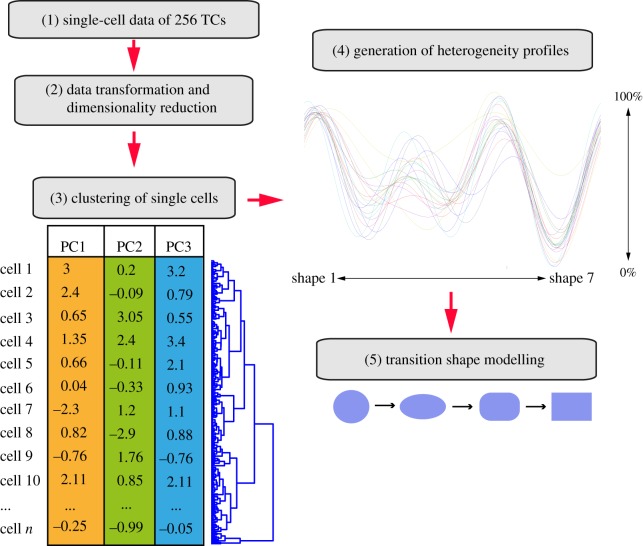
Figureu00a01.
Workflow for quantifying cellular shape space. (1) A high-dimensional dataset that measures 145 morphological features of 256 TCs and 12 061 cells is (2) log-transformed and projected into the first t...
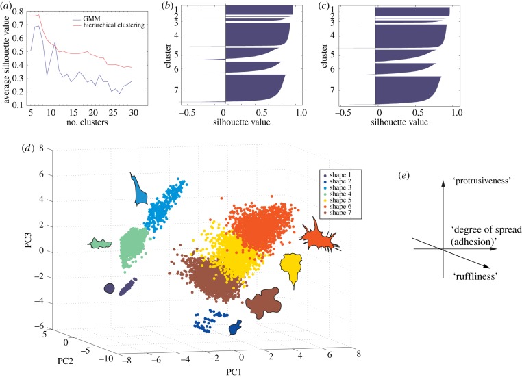
Figureu00a02.
Single-cell clustering. ( a ) Average silhouette value for different numbers of clusters using Gaussian mixture modelling (GMM) and hierarchical clustering. Higher averages represent better cluster qu...
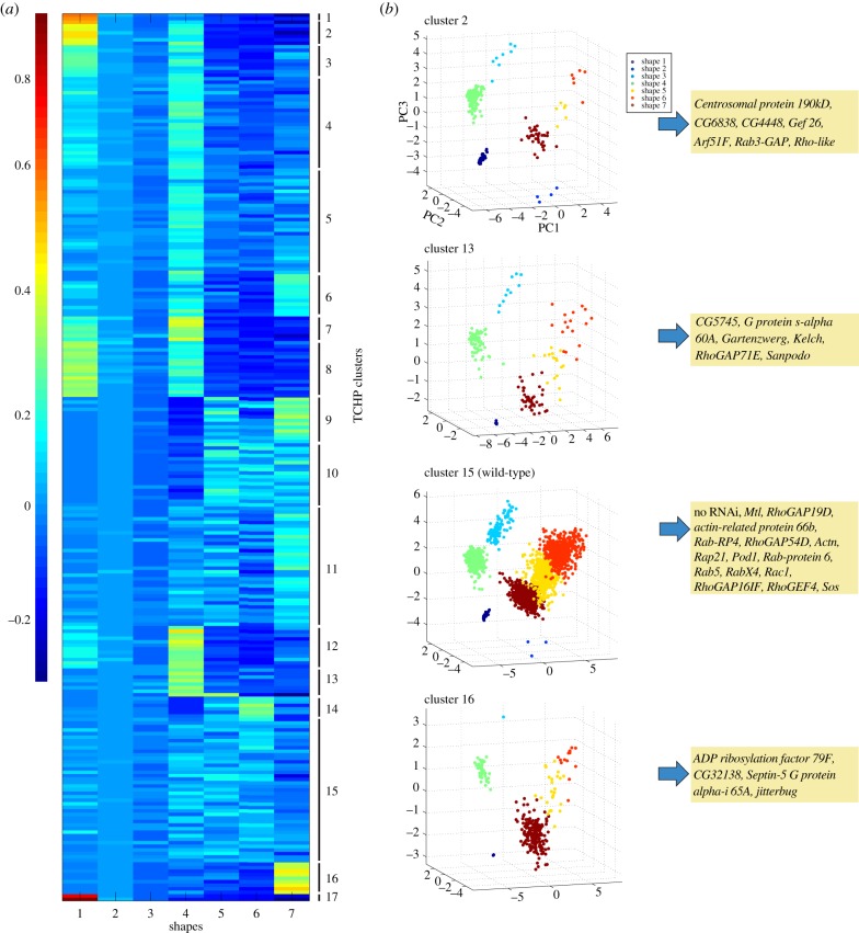
Figureu00a03.
Clustering of normalized TCHPs. ( a ) Heatmap of normalized TCHPs and their clustering based on the increase/decrease in different shapes. Red colour indicates high frequency of a shape in a TC, dark ...
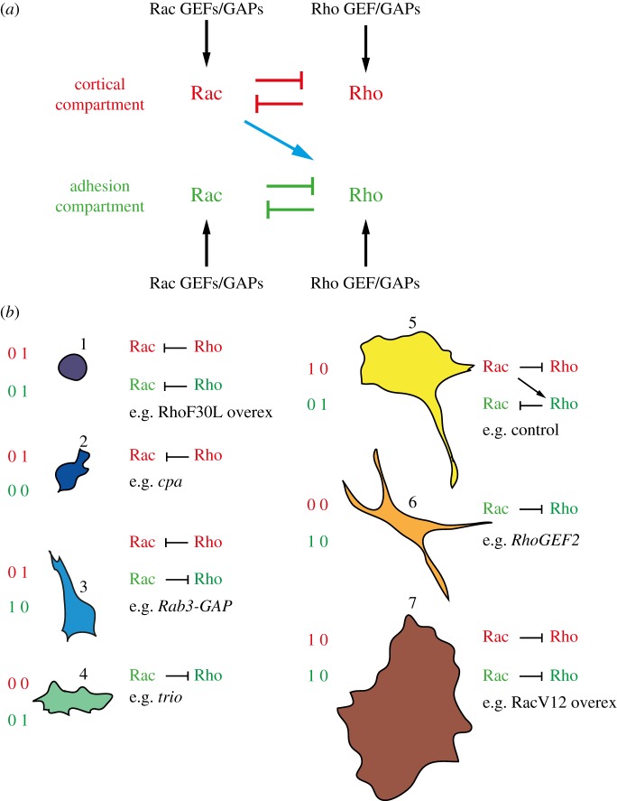
Figureu00a04.
A simple model of Rho/Rac activity in two distinct compartments exists in seven states. ( a ) We consider Rac and Rho activity in the cortical (red) and adhesion (green) compartments. In both compartm...
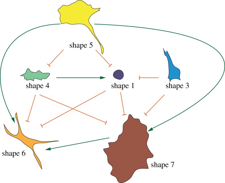
Figureu00a05.
Exploration of shape space by BG-2 cells occurs in a deterministic manner. Shape transition model: arrows describe the observed dependency of one shape on another. Green arrows describe dependencies w...
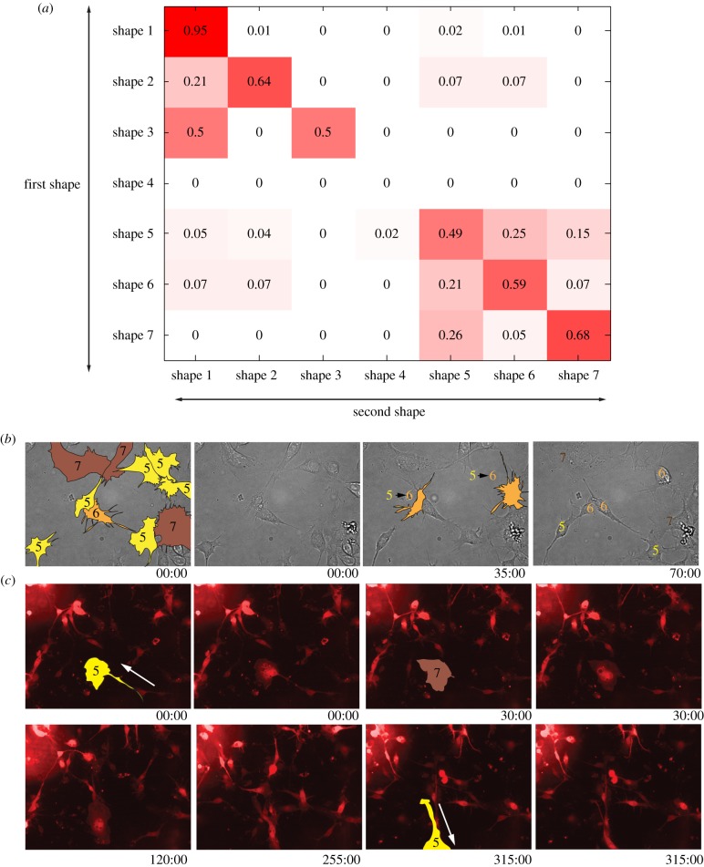
Figureu00a06.
Validation of the Bayesian model by live-cell imaging. ( a ) The probability of a cell transitioning from an initial shape (rows) to a subsequent shape (columns). The diagonal describes situations whe...
Figure images are served from the NIH/NLM PubMed Central Open Access Subset or Europe PMC; copyright remains with the publishers and authors.
💬 Discussion
0 commentsNo comments yet. Be the first to start a discussion!
Leave a Comment