Abstract
AbstractMacromolecular structure determination by electron cryo-microscopy (cryo-EM) is limited by the alignment of noisy images of individual particles. Because smaller particles have weaker signals, alignment errors impose size limitations on its applicability. Here, we explore how image alignment is improved by the application of deep learning to exploit prior knowledge about biological macromolecular structures that would otherwise be difficult to express mathematically. We train a denoising convolutional neural network on pairs of half-set reconstructions from the electron microscopy data bank (EMDB) and use this denoiser as an alternative to a commonly used smoothness prior. We demonstrate that this approach, which we call Blush regularization, yields better reconstructions than do existing algorithms, in particular for data with low signal-to-noise ratios. The reconstruction of a protein–nucleic acid complex with a molecular weight of 40 kDa, which was previously intractable, illustrates that denoising neural networks will expand the applicability of cryo-EM structure determination for a wide range of biological macromolecules.
🔬 Techniques
🧬 Organisms
💻 Software
✨ Fluorophores
🧪 Sample Preparation
🏭 Microscope Brands
💻 Software Details
💾 Data Repositories
🏛️ Research Organizations (ROR)
Affiliated research institutions:
📋 Methods
Rationale The noise2noise framework 8 facilitates the training of a denoising convolutional neural network in the absence of explicit access to ground-truth images. Instead, it relies on pairs of noisy images to extract information about their shared signal. Here, we present an application-specific approach that incorporates this aspect from the noise2noise framework. We trained a denoiser on a set of 422 pairs of noisy half-maps that we downloaded from the EMDB 30 . We selected only entries with reported resolutions higher than 4 Å for which both unfiltered half-maps were deposited. Maps with obvious artifacts, for example those associated with overfitting, and maps of a structure that was already present in the training set were eliminated during manual curation. We tailored data augmentation and training of the denoiser to integrate with the iterative expectation-maximization algorithm for cryo-EM reconstruction. All pairs of half-maps, documentclass[12pt]{minimal} usepackage{amsmath} usepackage{wasysym} usepackage{amsfonts} usepackage{amssymb} usepackage{amsbsy} usepackage{mathrsfs} usepackage{upgreek} setlength{oddsidemargin}{-69pt} begin{document}$${x}_{i}^{(k)}in {{mathbb{R}}}^{N}$$end{document} x i ( k ) ∈ R N , with k ∈ {0,1}, were re-scaled to a uniform voxel size of 1.5 Å, and augmented by generating new pairs documentclass[12pt]{minimal} usepackage{amsmath} usepackage{wasysym} usepackage{amsfonts} usepackage{amssymb} usepackage{amsbsy} usepackage{mathrsfs} usepackage{upgreek} setlength{oddsidemargin}{-69pt} begin{document}$${y}_{i}^{;k},{bar{y}}_{i}^{;k}in {{mathbb{R}}}^{N}$$end{document} y i k , ȳ i k ∈ R N : 1 documentclass[12pt]{minimal} usepackage{amsmath} usepackage{wasysym} usepackage{amsfonts} usepackage{amssymb} usepackage{amsbsy} usepackage{mathrsfs} usepackage{upgreek} setlength{oddsidemargin}{-69pt} begin{document}$${y}_{i}^{(k)}={{{{rm{H}}}}}_{C,;A}left[{x}_{i}^{(1-k)}+{e}^{(1-k)}right],$$end{document} y i ( k ) = H C , A x i ( 1 − k ) + e ( 1 − k ) , 2 documentclass[12pt]{minimal} usepackage{amsmath} usepackage{wasysym} usepackage{amsfonts} usepackage{amssymb} usepackage{amsbsy} usepackage{mathrsfs} usepackage{upgreek} setlength{oddsidemargin}{-69pt} begin{document}$${bar{y}}_{i}^{(k)}={{{{rm{H}}}}}_{bar{C},;A}left[{x}_{i}^{(k)}odot {M}_{i}+{{{rm{h}}}}left({x}_{i}^{(k)}right)odot (1-{M}_{i})right],$$end{document} ȳ i ( k ) = H C ¯ , A x i ( k ) ⊙ M i + h x i ( k ) ⊙ ( 1 − M i ) , where documentclass[12pt]{minimal} usepackage{amsmath} usepackage{wasysym} usepackage{amsfonts} usepackage{amssymb} usepackage{amsbsy} usepackage{mathrsfs} usepackage{upgreek} setlength{oddsidemargin}{-69pt} begin{document}$$ein {{mathbb{R}}}^{N}$$end{document} e ∈ R N is random colored noise, M i ∈ [0, 1] N is a smooth mask encapsulating the molecules of interest, ⊙ represents voxel-wise multiplication and h(.) is a low-pass filter to 15 Å. H C , A [.] applies an anisotropic Gaussian filter with covariance matrix C , an affine transform A that includes rotation and translation, a crop to a patch of 64 3 voxels and a voxel-value standardization. Data augmentation was achieved through random assignments of documentclass[12pt]{minimal} usepackage{amsmath} usepackage{wasysym} usepackage{amsfonts} usepackage{amssymb} usepackage{amsbsy} usepackage{mathrsfs} usepackage{upgreek} setlength{oddsidemargin}{-69pt} begin{document}$$C,bar{C},A,e$$end{document} C , C ¯ , A , e and r . By using a range of resolution cut-offs for C and documentclass[12pt]{minimal} usepackage{amsmath} usepackage{wasysym} usepackage{amsfonts} usepackage{amssymb} usepackage{amsbsy} usepackage{mathrsfs} usepackage{upgreek} setlength{oddsidemargin}{-69pt} begin{document}$$bar{C}$$end{document} C ¯ , the denoiser explicitly learns to handle maps with varying resolutions. This is necessary for its application inside the iterative expectation-maximization algorithm, which typically starts at relatively low resolutions and gradually progresses to higher resolutions. Although using a lower resolution cut-off for C than for documentclass[12pt]{minimal} usepackage{amsmath} usepackage{wasysym} usepackage{amsfonts} usepackage{amssymb} usepackage{amsbsy} usepackage{mathrsfs} usepackage{upgreek} setlength{oddsidemargin}{-69pt} begin{document}$$bar{C}$$end{document} C ¯ could have produced a network that enhances the resolution of the half-maps, similar to deblurring networks 31 , we opted not to do so to minimize the risk of hallucinations in high-resolution features. Using different degrees of anisotropy in C and documentclass[12pt]{minimal} usepackage{amsmath} usepackage{wasysym} usepackage{amsfonts} usepackage{amssymb} usepackage{amsbsy} usepackage{mathrsfs} usepackage{upgreek} setlength{oddsidemargin}{-69pt} begin{document}$$bar{C}$$end{document} C ¯ , the denoiser learns to deal with the artifacts that arise from non-uniform orientational distributions, and random orientations and affine transformations in A lead to invariance with respect to rotations, translations and intensity scale. Although initial versions of our training protocol did not include masks, we observed that the resulting networks would learn to smoothen densities in disordered regions, such as the solvent or detergent micelles, which would improve image alignments. To amplify these effects, we then implemented the supervised masking approach with M i and h(.). By filling disordered regions with a 15-Å-resolution low-pass filtered version of the map, as opposed to a straightforward voxel-wise multiplication with the mask M i , higher density values in regions with disordered molecules, such as detergent micelles, are maintained. By re-scaling all maps to a common voxel size of 1.5 Å, and then cropping maps to patches of 64 3 voxels, the network can be trained on and applied to maps of any size. To apply the denoiser to maps that are larger than one patch, overlapping patches can be denoised independently. Training the denoiser Our denoiser ( f θ ) consists of a U-net with approximately 13 million trainable parameters ( θ ) (Fig. 1 ). It is trained using residual learning 32 and with a dropout rate of 50% (ref. 33 ). Instance normalization 34 is used to handle small mini-batches ( documentclass[12pt]{minimal} usepackage{amsmath} usepackage{wasysym} usepackage{amsfonts} usepackage{amssymb} usepackage{amsbsy} usepackage{mathrsfs} usepackage{upgreek} setlength{oddsidemargin}{-69pt} begin{document}$${{{mathcal{B}}}}$$end{document} B ), with b = 8 samples from the training dataset, during training. We minimize the following loss: 3 documentclass[12pt]{minimal} usepackage{amsmath} usepackage{wasysym} usepackage{amsfonts} usepackage{amssymb} usepackage{amsbsy} usepackage{mathrsfs} usepackage{upgreek} setlength{oddsidemargin}{-69pt} begin{document}$${{{mathcal{L}}}}=frac{1}{2b}mathop{sum}limits_{iin {{{mathcal{B}}}}}mathop{sum}limits_{kin {0,1}}{leftVert; {bar{y}}_{i}^{(k)}-{f}_{theta }left({{{{rm{R}}}}}_{r}left[;{f}_{theta },{y}_{i}^{(k)}right]right)rightVert }^{2},$$end{document} L = 1 2 b ∑ i ∈ B ∑ k ∈ { 0 , 1 } ȳ i ( k ) − f θ R r f θ , y i ( k ) 2 , where R r [ f θ , y ] returns the output of the denoiser f θ after recursively calling it r ∈ {0, …, 5} times with documentclass[12pt]{minimal} usepackage{amsmath} usepackage{wasysym} usepackage{amsfonts} usepackage{amssymb} usepackage{amsbsy} usepackage{mathrsfs} usepackage{upgreek} setlength{oddsidemargin}{-69pt} begin{document}$${y}_{i}^{;k}$$end{document} y i k as the initial input. This enables the denoiser to recognize and suppress artifacts brought about by its repeated usage, thereby limiting the amplification of artifacts in the reconstruction that are introduced by the denoiser during subsequent iterations of the expectation-maximization algorithm 7 . Training for 950,000 steps took six days using a single Nvidia A100 GPU. Iterative denoising with spectral trailing We refer to the application of our pre-trained denoiser within the iterative expectation-maximization algorithm as Blush regularization. In our original work, with simulated data, we incorporated the denoiser into the L 2 regularization in the M-step, on the basis of the approximation that the prior function is ‘close’ to a Gaussian 7 . In this work, we do not make formal claims about the role of the denoiser within a Bayesian framework. Instead, our approach is motivated by empirical observations. Although one effect of the denoiser is that it tends to dampen Fourier components at higher spatial frequencies, the amount by which it does so is not well defined. Therefore, we use a heuristic method, here referred to as spectral trailing, to prevent overfitting in 3D autorefinement and multi-body refinement. First, we calculate the FSC between two independently refined half-maps before the denoiser is applied, and determine the ρ value at which the solvent-corrected FSC drops below 0.143. We then apply the denoiser to both half-maps and subsequently apply a low-pass filter at a spatial frequency that is two Fourier shells (each shell is one Fourier voxel wide) lower than ρ . If ρ exceeds the Nyquist frequency of the denoiser, here set to 3 Å, the remaining Fourier shells at higher frequencies are populated with the reconstruction from the standard regularization in Fourier space. The resulting denoised, low-pass-filtered maps are then used as references for alignment in the next iteration. The denoiser is not applied to the output of the final refinement step. Blush regularization has been implemented in the open-source software RELION-5, using a combination of C++ and PyTorch. It can be used for 3D classification, multi-body refinement and 3D autorefinement jobs, including those for particles with point-group or helical symmetry. For 3D classification for data that are separated into independent half-sets, the filtered map from the regularized likelihood approach is used as input for the denoiser. No additional low-pass filtering is applied. In this job type, the denoiser is also applied in the last iteration. Reporting summary Further information on research design is available in the Nature Portfolio Reporting Summary linked to this article.
Show full methods section
Rationale The noise2noise framework 8 facilitates the training of a denoising convolutional neural network in the absence of explicit access to ground-truth images. Instead, it relies on pairs of noisy images to extract information about their shared signal. Here, we present an application-specific approach that incorporates this aspect from the noise2noise framework. We trained a denoiser on a set of 422 pairs of noisy half-maps that we downloaded from the EMDB 30 . We selected only entries with reported resolutions higher than 4 Å for which both unfiltered half-maps were deposited. Maps with obvious artifacts, for example those associated with overfitting, and maps of a structure that was already present in the training set were eliminated during manual curation. We tailored data augmentation and training of the denoiser to integrate with the iterative expectation-maximization algorithm for cryo-EM reconstruction. All pairs of half-maps, documentclass[12pt]{minimal} usepackage{amsmath} usepackage{wasysym} usepackage{amsfonts} usepackage{amssymb} usepackage{amsbsy} usepackage{mathrsfs} usepackage{upgreek} setlength{oddsidemargin}{-69pt} begin{document}$${x}_{i}^{(k)}in {{mathbb{R}}}^{N}$$end{document} x i ( k ) ∈ R N , with k ∈ {0,1}, were re-scaled to a uniform voxel size of 1.5 Å, and augmented by generating new pairs documentclass[12pt]{minimal} usepackage{amsmath} usepackage{wasysym} usepackage{amsfonts} usepackage{amssymb} usepackage{amsbsy} usepackage{mathrsfs} usepackage{upgreek} setlength{oddsidemargin}{-69pt} begin{document}$${y}_{i}^{;k},{bar{y}}_{i}^{;k}in {{mathbb{R}}}^{N}$$end{document} y i k , ȳ i k ∈ R N : 1 documentclass[12pt]{minimal} usepackage{amsmath} usepackage{wasysym} usepackage{amsfonts} usepackage{amssymb} usepackage{amsbsy} usepackage{mathrsfs} usepackage{upgreek} setlength{oddsidemargin}{-69pt} begin{document}$${y}_{i}^{(k)}={{{{rm{H}}}}}_{C,;A}left[{x}_{i}^{(1-k)}+{e}^{(1-k)}right],$$end{document} y i ( k ) = H C , A x i ( 1 − k ) + e ( 1 − k ) , 2 documentclass[12pt]{minimal} usepackage{amsmath} usepackage{wasysym} usepackage{amsfonts} usepackage{amssymb} usepackage{amsbsy} usepackage{mathrsfs} usepackage{upgreek} setlength{oddsidemargin}{-69pt} begin{document}$${bar{y}}_{i}^{(k)}={{{{rm{H}}}}}_{bar{C},;A}left[{x}_{i}^{(k)}odot {M}_{i}+{{{rm{h}}}}left({x}_{i}^{(k)}right)odot (1-{M}_{i})right],$$end{document} ȳ i ( k ) = H C ¯ , A x i ( k ) ⊙ M i + h x i ( k ) ⊙ ( 1 − M i ) , where documentclass[12pt]{minimal} usepackage{amsmath} usepackage{wasysym} usepackage{amsfonts} usepackage{amssymb} usepackage{amsbsy} usepackage{mathrsfs} usepackage{upgreek} setlength{oddsidemargin}{-69pt} begin{document}$$ein {{mathbb{R}}}^{N}$$end{document} e ∈ R N is random colored noise, M i ∈ [0, 1] N is a smooth mask encapsulating the molecules of interest, ⊙ represents voxel-wise multiplication and h(.) is a low-pass filter to 15 Å. H C , A [.] applies an anisotropic Gaussian filter with covariance matrix C , an affine transform A that includes rotation and translation, a crop to a patch of 64 3 voxels and a voxel-value standardization. Data augmentation was achieved through random assignments of documentclass[12pt]{minimal} usepackage{amsmath} usepackage{wasysym} usepackage{amsfonts} usepackage{amssymb} usepackage{amsbsy} usepackage{mathrsfs} usepackage{upgreek} setlength{oddsidemargin}{-69pt} begin{document}$$C,bar{C},A,e$$end{document} C , C ¯ , A , e and r . By using a range of resolution cut-offs for C and documentclass[12pt]{minimal} usepackage{amsmath} usepackage{wasysym} usepackage{amsfonts} usepackage{amssymb} usepackage{amsbsy} usepackage{mathrsfs} usepackage{upgreek} setlength{oddsidemargin}{-69pt} begin{document}$$bar{C}$$end{document} C ¯ , the denoiser explicitly learns to handle maps with varying resolutions. This is necessary for its application inside the iterative expectation-maximization algorithm, which typically starts at relatively low resolutions and gradually progresses to higher resolutions. Although using a lower resolution cut-off for C than for documentclass[12pt]{minimal} usepackage{amsmath} usepackage{wasysym} usepackage{amsfonts} usepackage{amssymb} usepackage{amsbsy} usepackage{mathrsfs} usepackage{upgreek} setlength{oddsidemargin}{-69pt} begin{document}$$bar{C}$$end{document} C ¯ could have produced a network that enhances the resolution of the half-maps, similar to deblurring networks 31 , we opted not to do so to minimize the risk of hallucinations in high-resolution features. Using different degrees of anisotropy in C and documentclass[12pt]{minimal} usepackage{amsmath} usepackage{wasysym} usepackage{amsfonts} usepackage{amssymb} usepackage{amsbsy} usepackage{mathrsfs} usepackage{upgreek} setlength{oddsidemargin}{-69pt} begin{document}$$bar{C}$$end{document} C ¯ , the denoiser learns to deal with the artifacts that arise from non-uniform orientational distributions, and random orientations and affine transformations in A lead to invariance with respect to rotations, translations and intensity scale. Although initial versions of our training protocol did not include masks, we observed that the resulting networks would learn to smoothen densities in disordered regions, such as the solvent or detergent micelles, which would improve image alignments. To amplify these effects, we then implemented the supervised masking approach with M i and h(.). By filling disordered regions with a 15-Å-resolution low-pass filtered version of the map, as opposed to a straightforward voxel-wise multiplication with the mask M i , higher density values in regions with disordered molecules, such as detergent micelles, are maintained. By re-scaling all maps to a common voxel size of 1.5 Å, and then cropping maps to patches of 64 3 voxels, the network can be trained on and applied to maps of any size. To apply the denoiser to maps that are larger than one patch, overlapping patches can be denoised independently. Training the denoiser Our denoiser ( f θ ) consists of a U-net with approximately 13 million trainable parameters ( θ ) (Fig. 1 ). It is trained using residual learning 32 and with a dropout rate of 50% (ref. 33 ). Instance normalization 34 is used to handle small mini-batches ( documentclass[12pt]{minimal} usepackage{amsmath} usepackage{wasysym} usepackage{amsfonts} usepackage{amssymb} usepackage{amsbsy} usepackage{mathrsfs} usepackage{upgreek} setlength{oddsidemargin}{-69pt} begin{document}$${{{mathcal{B}}}}$$end{document} B ), with b = 8 samples from the training dataset, during training. We minimize the following loss: 3 documentclass[12pt]{minimal} usepackage{amsmath} usepackage{wasysym} usepackage{amsfonts} usepackage{amssymb} usepackage{amsbsy} usepackage{mathrsfs} usepackage{upgreek} setlength{oddsidemargin}{-69pt} begin{document}$${{{mathcal{L}}}}=frac{1}{2b}mathop{sum}limits_{iin {{{mathcal{B}}}}}mathop{sum}limits_{kin {0,1}}{leftVert; {bar{y}}_{i}^{(k)}-{f}_{theta }left({{{{rm{R}}}}}_{r}left[;{f}_{theta },{y}_{i}^{(k)}right]right)rightVert }^{2},$$end{document} L = 1 2 b ∑ i ∈ B ∑ k ∈ { 0 , 1 } ȳ i ( k ) − f θ R r f θ , y i ( k ) 2 , where R r [ f θ , y ] returns the output of the denoiser f θ after recursively calling it r ∈ {0, …, 5} times with documentclass[12pt]{minimal} usepackage{amsmath} usepackage{wasysym} usepackage{amsfonts} usepackage{amssymb} usepackage{amsbsy} usepackage{mathrsfs} usepackage{upgreek} setlength{oddsidemargin}{-69pt} begin{document}$${y}_{i}^{;k}$$end{document} y i k as the initial input. This enables the denoiser to recognize and suppress artifacts brought about by its repeated usage, thereby limiting the amplification of artifacts in the reconstruction that are introduced by the denoiser during subsequent iterations of the expectation-maximization algorithm 7 . Training for 950,000 steps took six days using a single Nvidia A100 GPU. Iterative denoising with spectral trailing We refer to the application of our pre-trained denoiser within the iterative expectation-maximization algorithm as Blush regularization. In our original work, with simulated data, we incorporated the denoiser into the L 2 regularization in the M-step, on the basis of the approximation that the prior function is ‘close’ to a Gaussian 7 . In this work, we do not make formal claims about the role of the denoiser within a Bayesian framework. Instead, our approach is motivated by empirical observations. Although one effect of the denoiser is that it tends to dampen Fourier components at higher spatial frequencies, the amount by which it does so is not well defined. Therefore, we use a heuristic method, here referred to as spectral trailing, to prevent overfitting in 3D autorefinement and multi-body refinement. First, we calculate the FSC between two independently refined half-maps before the denoiser is applied, and determine the ρ value at which the solvent-corrected FSC drops below 0.143. We then apply the denoiser to both half-maps and subsequently apply a low-pass filter at a spatial frequency that is two Fourier shells (each shell is one Fourier voxel wide) lower than ρ . If ρ exceeds the Nyquist frequency of the denoiser, here set to 3 Å, the remaining Fourier shells at higher frequencies are populated with the reconstruction from the standard regularization in Fourier space. The resulting denoised, low-pass-filtered maps are then used as references for alignment in the next iteration. The denoiser is not applied to the output of the final refinement step. Blush regularization has been implemented in the open-source software RELION-5, using a combination of C++ and PyTorch. It can be used for 3D classification, multi-body refinement and 3D autorefinement jobs, including those for particles with point-group or helical symmetry. For 3D classification for data that are separated into independent half-sets, the filtered map from the regularized likelihood approach is used as input for the denoiser. No additional low-pass filtering is applied. In this job type, the denoiser is also applied in the last iteration. Reporting summary Further information on research design is available in the Nature Portfolio Reporting Summary linked to this article.
Online content Any methods, additional references, Nature Portfolio reporting summaries, source data, extended data, supplementary information, acknowledgements, peer review information; details of author contributions and competing interests; and statements of data and code availability are available at 10.1038/s41592-024-02304-8.
Supplementary information Reporting Summary Peer Review File
Supplementary information The online version contains supplementary material available at 10.1038/s41592-024-02304-8.
📊 Figures
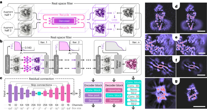
Fig. 1
Schematic illustration of Blush regularization and slices of example volumes.
a , Training procedure, showing two passes for both half-maps and recycling of the denoiser output (in pink), with calculation of a mean squared error (L2) loss. b , Iterative reconstruction with spec...
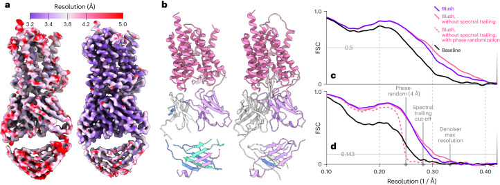
Fig. 2
Single-particle reconstruction of the PfCRT dataset.
a , Maps colored by local resolution, comparing the baseline reconstruction (left) and the reconstruction after Blush regularization (right). b , Automated atomic modeling by ModelAngelo for the basel...
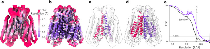
Fig. 3
Single-particle reconstruction of the Ste2 dataset.
a , b , Reconstructions of the Ste2 dataset, colored by local resolution, comparing the baseline reconstruction ( a ) and the reconstruction after Blush regularization ( b ). c , d , Automated atomic ...
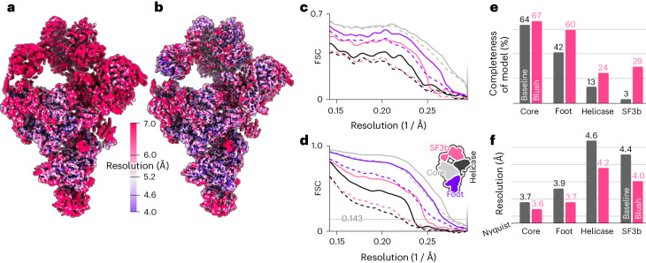
Fig. 4
Multi-body reconstruction of the spliceosome dataset.
a , b , Combined maps of the individual bodies, colored by local resolution, comparing the baseline reconstruction ( a ) and the reconstruction after Blush regularization ( b ). c , FSCs between the m...
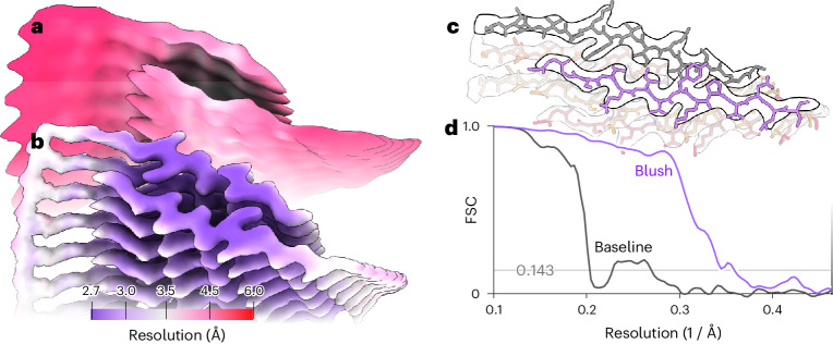
Fig. 5
Helical reconstruction of the FIA, colored by local resolution, for the baseline.
a , b , Maps of the baseline reconstruction ( a ) and after application of Blush regularization ( b ). c , Automated atomic modeling by ModelAngelo, comprising tau residues 302u2013316. d , Solvent-co...
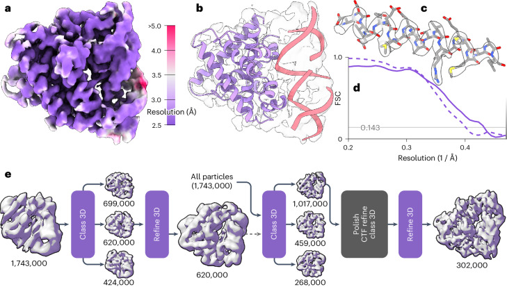
Fig. 6
Single-particle reconstruction of the Aca2u2013RNA complex with a molecular weight of 40 kDa.
a , Local resolution of the reconstruction with Blush regularization. b , Automated atomic model assignment with ModelAngelo. c , Detailed view of an u03b1-helical segment in the reconstructed map and...
Figure images are served from the NIH/NLM PubMed Central Open Access Subset or Europe PMC; copyright remains with the publishers and authors.
💬 Discussion
0 commentsNo comments yet. Be the first to start a discussion!
Leave a Comment