Abstract
Increasingly, cryo-electron microscopy (cryo-EM) is used to determine the structures of RNA-protein assemblies, but nearly all maps determined with this method have biologically important regions where the local resolution does not permit RNA coordinate tracing. To address these omissions, we present de novo ribonucleoprotein modeling in real space through assembly of fragments together with experimental density in Rosetta (DRRAFTER). We show that DRRAFTER recovers near-native models for a diverse benchmark set of RNA-protein complexes including the spliceosome, mitochondrial ribosome, and CRISPR-Cas9-sgRNA complexes; rigorous blind tests include yeast U1 snRNP and spliceosomal P complex maps. Additionally, to aid in model interpretation, we present a method for reliable in situ estimation of DRRAFTER model accuracy. Finally, we apply DRRAFTER to recently determined maps of telomerase, the HIV-1 reverse transcriptase initiation complex, and the packaged MS2 genome, demonstrating the acceleration of accurate model building in challenging cases.
🔬 Techniques
🧬 Organisms
🧪 Sample Preparation
💻 Software Details
💾 Data Repositories
🏛️ Research Organizations (ROR)
Affiliated research institutions:
📋 Methods
The DRRAFTER pipeline For each system, all available structures of individual proteins were collected from the PDB and then fit into the cryoEM density map in Chimera using the “Fit in Map” function [ 51 ]. Ideal A-form RNA helices were built with the Rosetta tool, rna_helix.py, and then fit into the maps in Chimera [ 51 ]. Following conventional protocols [ 9 – 12 ], these steps were performed manually, but completed rapidly (minutes per structure). Regions with missing RNA coordinates were identified and subdivided by visual inspection. The surrounding RNA helices and proteins were extracted from the overall model of the RNP and used as the input to the Rosetta DRRAFTER run. The Rosetta stage consists of a modified version of the FARFAR method, run through the Rosetta rna_denovo application [ 52 , 53 ]. The method was updated so that both proteins and density maps can be included. There are two stages to this protocol. First, a low resolution Monte Carlo stage, which includes standard RNA fragment insertion moves to fold the RNA, now allows docking moves that optimize the placement of RNA helices and proteins. Docking moves for RNA helices include rotations and translations about the helical axis, in addition to the standard random rigid body perturbations. During this stage, the proteins are treated as rigid bodies. Each conformation is scored with the low-resolution RNA-protein potential in Rosetta [ 54 ], augmented by the “elec_dens_fast” score term, which scores the agreement between the map and model [ 55 ]. After the low-resolution stage, the structure goes through full-atom refinement. First, the structure is subjected to energy minimization in which the RNA as well as the protein sidechains within a 20.0 Å distance of any RNA atom are allowed to move. Then, the structure is further refined through single residue fragment insertions, sidechain packing, and small rigid body perturbations. The structure is then subjected to a second round of energy minimization. Scoring during these phases is performed with the full-atom Rosetta energy function, which includes terms that describe hydrogen bonding, electrostatics, torsional energy, van der Waals interactions and solvation, and is also supplemented with the density score term elec_dens_fast [ 55 , 56 ]. This score function is available within Rosetta as “rna_hires_with_protein.wts”. The top ten models are output from the run, with the centroid model highlighted, to be visually inspected and to allow final manual selection. The DRRAFTER code is freely available to academic users as part of the Rosetta software package in releases after March 14, 2018 excluding Rosetta 3.9 ( www.rosettacommons.org ) and is automatically compiled along with ERRASER, which is already in routine use for RNA and RNP cryoEM. An example Rosetta command line is as follows: DRRAFTER.py -fasta fasta.txt -secstruct secstruct.txt -start_struct my_starting_structure.pdb -map_file my_cryoEM_map.mrc -map_reso 7.0 -residues_to_model A:20–30 -job_name my_drrafter_run where fasta.txt is a FASTA file listing the full sequence of the complex, secstruct.txt is a file containing the secondary structure in dot bracket notation (with dots for protein residues), -residues_to_model (here given a value of A:20–30) specifies the residues that should be built in the DRRAFTER run, my_starting_structure.pdb is the PDB file containing all fit protein structures and RNA helices, -map_file specifies the density map, -map_reso specifies the resolution of the map, and -job_name specifies a name for the run (which controls the names of the output files). Documentation and a demo are available at www.rosettacommons.org . Modeling convergence was calculated by taking the average of the pairwise RMSDs over the RNA region being modeled for the best ten scoring DRRAFTER models. An example command line to calculate convergence and corresponding error estimates is as follows: DRRAFTER.py -estimate_error -final_structures model_1.pdb model_2.pdb model_3.pdb model_4.pdb model_5.pdb model_6.pdb model_7.pdb model_8.pdb model_9.pdb model_10.pdb Approximately 3000 DRRAFTER models were generated in all cases, and the top ten scoring were then subjected to the PHENIX-ERRASER pipeline [ 20 ]. For the PHENIX runs, secondary structure restraints were automatically generated using phenix.secondary_structure_restraints and applied during refinement with phenix.real_space_refine. Additionally, coordinate restraints were applied for all residues in RNA helices. During the ERRASER runs, the first base pair of each RNA helix was kept fixed, as well as any residues contacting a protein surface, or near enough that ERRASER introduced protein-RNA clashes if the residue was not kept fixed.
Show full methods section
The DRRAFTER pipeline For each system, all available structures of individual proteins were collected from the PDB and then fit into the cryoEM density map in Chimera using the “Fit in Map” function [ 51 ]. Ideal A-form RNA helices were built with the Rosetta tool, rna_helix.py, and then fit into the maps in Chimera [ 51 ]. Following conventional protocols [ 9 – 12 ], these steps were performed manually, but completed rapidly (minutes per structure). Regions with missing RNA coordinates were identified and subdivided by visual inspection. The surrounding RNA helices and proteins were extracted from the overall model of the RNP and used as the input to the Rosetta DRRAFTER run. The Rosetta stage consists of a modified version of the FARFAR method, run through the Rosetta rna_denovo application [ 52 , 53 ]. The method was updated so that both proteins and density maps can be included. There are two stages to this protocol. First, a low resolution Monte Carlo stage, which includes standard RNA fragment insertion moves to fold the RNA, now allows docking moves that optimize the placement of RNA helices and proteins. Docking moves for RNA helices include rotations and translations about the helical axis, in addition to the standard random rigid body perturbations. During this stage, the proteins are treated as rigid bodies. Each conformation is scored with the low-resolution RNA-protein potential in Rosetta [ 54 ], augmented by the “elec_dens_fast” score term, which scores the agreement between the map and model [ 55 ]. After the low-resolution stage, the structure goes through full-atom refinement. First, the structure is subjected to energy minimization in which the RNA as well as the protein sidechains within a 20.0 Å distance of any RNA atom are allowed to move. Then, the structure is further refined through single residue fragment insertions, sidechain packing, and small rigid body perturbations. The structure is then subjected to a second round of energy minimization. Scoring during these phases is performed with the full-atom Rosetta energy function, which includes terms that describe hydrogen bonding, electrostatics, torsional energy, van der Waals interactions and solvation, and is also supplemented with the density score term elec_dens_fast [ 55 , 56 ]. This score function is available within Rosetta as “rna_hires_with_protein.wts”. The top ten models are output from the run, with the centroid model highlighted, to be visually inspected and to allow final manual selection. The DRRAFTER code is freely available to academic users as part of the Rosetta software package in releases after March 14, 2018 excluding Rosetta 3.9 ( www.rosettacommons.org ) and is automatically compiled along with ERRASER, which is already in routine use for RNA and RNP cryoEM. An example Rosetta command line is as follows: DRRAFTER.py -fasta fasta.txt -secstruct secstruct.txt -start_struct my_starting_structure.pdb -map_file my_cryoEM_map.mrc -map_reso 7.0 -residues_to_model A:20–30 -job_name my_drrafter_run where fasta.txt is a FASTA file listing the full sequence of the complex, secstruct.txt is a file containing the secondary structure in dot bracket notation (with dots for protein residues), -residues_to_model (here given a value of A:20–30) specifies the residues that should be built in the DRRAFTER run, my_starting_structure.pdb is the PDB file containing all fit protein structures and RNA helices, -map_file specifies the density map, -map_reso specifies the resolution of the map, and -job_name specifies a name for the run (which controls the names of the output files). Documentation and a demo are available at www.rosettacommons.org . Modeling convergence was calculated by taking the average of the pairwise RMSDs over the RNA region being modeled for the best ten scoring DRRAFTER models. An example command line to calculate convergence and corresponding error estimates is as follows: DRRAFTER.py -estimate_error -final_structures model_1.pdb model_2.pdb model_3.pdb model_4.pdb model_5.pdb model_6.pdb model_7.pdb model_8.pdb model_9.pdb model_10.pdb Approximately 3000 DRRAFTER models were generated in all cases, and the top ten scoring were then subjected to the PHENIX-ERRASER pipeline [ 20 ]. For the PHENIX runs, secondary structure restraints were automatically generated using phenix.secondary_structure_restraints and applied during refinement with phenix.real_space_refine. Additionally, coordinate restraints were applied for all residues in RNA helices. During the ERRASER runs, the first base pair of each RNA helix was kept fixed, as well as any residues contacting a protein surface, or near enough that ERRASER introduced protein-RNA clashes if the residue was not kept fixed.
Model analysis
RMSDs (reported in Supplementary Table 1 ) were calculated over RNA heavy atoms after initial alignment over protein heavy atoms. These calculations were carried out in Rosetta and Pymol. RMSDs for previously modeled coordinates in the spliceosomal tri-snRNP were calculated for protein structures that had been fit into the lower-resolution (5.9 Å) density map in Chimera following the description in the methods section of the original paper [ 9 ] versus the high-resolution coordinates of the corresponding proteins in PDB ID 5GAN [ 35 ]. Homologous protein structures that were docked into the lower-resolution map were omitted from this calculation. For the mitoribosome, RMSDs were calculated between the coordinates deposited with the lower-resolution (4.9 Å) map (PDB ID: 4CE4) and the high-resolution (3.4 Å) map (PDB ID: 4V1A and 4V19) for proteins present in both as well as for RNA regions that could not have been modeled by simple threading of the E. coli ribosome structure. For the Cas9-sgRNA complex, the protein coordinates were taken from the crystal structure of CRISPR-Cas9 in complex with sgRNA and double stranded DNA (PDB ID 5F9R) and broken up into domains, and each of these was individually fit into the cryoEM density map [ 36 ]. RMSDs between these regions and the high-resolution crystal structure (PDB ID 4ZT0) were calculated. Local map resolution was calculated with Resmap [ 7 ], then loaded into Chimera along with the corresponding high-resolution coordinates. The “Values at Atom Positions” tool in Chimera was used to find the local resolution at the positions of each of the atoms in the high-resolution structure. The values at the positions of all of the RNA atoms for the region being modeled were averaged (with a python script) to give the local resolution for that region. Best-fit lines describing the upper and lower bounds of DRRAFTER model accuracy versus local resolution ( Figure 3a ) were calculated using the minimum RMSD values (lower bound) or 90 th percentile RMSD values (upper bound) in each 1 Å bin ranging from 2.5 to 12.5 Å local resolution. Real-space correlation coefficients were calculated for RNA coordinates being modeled only (surrounding proteins were not included to facilitate comparison between high- and low-resolution coordinates) using the PHENIX tool phenix.get_cc_mtz_pdb with fix_xyz=True and scale=True. The “Map correlation in region of model” was reported. Figures were generated with Pymol and UCSF Chimera. The versions of all software used in this study are listed in the Life Sciences Reporting Summary.
Statistics
Pearson’s correlation coefficients were calculated for local resolution (determined as described above) versus model accuracy for a total of 128 models, of which 30 were DRRAFTER models built into simulated maps, 25 were DRRAFTER models built into experimental maps, 6 were blind DRRAFTER models built into experimental maps, and 67 were previously modeled low-resolution protein and RNA coordinates. Pearson’s correlation coefficients were also calculated for the mean, median, and best model accuracy out of the top ten scoring DRRAFTER models versus modeling convergence (calculated as described above) for 61 systems of which 30 were DRRAFTER models built into simulated maps, 25 were DRRAFTER models built into experimental maps, and 6 were blind DRRAFTER models built into experimental maps. Two-tailed p-values are reported for all correlation coefficients. Simulated benchmark Ten systems were chosen from the nonredundant set of RNA-protein complexes with corresponding unbound protein structures available, described in [ 57 ]. The specific systems were selected manually to represent a diversity of types of RNA-protein interactions (unbound protein structures listed in parentheses): 1DFU (1B75), 1B7F (3SXL), 1JBS (1AQZ), 1P6V (1K8H), 1WPU (1WPV), 1WSU (1LVA), 2ASB (1K0R), 2BH2 (1UWV), 2QUX (2QUD), and 3BX2 (3BWT). For each of these systems, density maps were simulated at 3.0 Å, 5.0 Å, and 7.0 Å resolution with the pdb2vol tool in the Situs package [ 58 ]. Unbound protein structures (listed above) were fit into the simulated density maps using Chimera’s Fit in Map tool. Ideal RNA helices for helical segments of RNA were generated with rna_helix.py in Rosetta and then fit into the maps using Chimera’s Fit in Map tool. For systems that contained only single-stranded RNA, an ideal A-form nucleotide was fit approximately into the map – throughout the later DRRAFTER simulation, it was allowed to change its conformation and orientation within the map. The remaining RNA residues were also built with the DRRAFTER protocol in Rosetta. The full protein structures were included in the simulations, and were allowed to dock as rigid bodies within the density map. The ideal RNA helices were also subjected to docking within the map to optimize their final placement.
Spliceosomal tri-snRNP modeling
All proteins listed in Extended Data Table 1 of the original paper [ 9 ] were fit into the full tri-snRNP density map (EMD 2966), as well as the structure of the C-terminal fragment of PRP3, which had since been solved (PDB ID: 4YHU) [ 59 ]. Ideal RNA helices were fit into the map for all helical parts of the three regions modeled: the U5 snRNA three-way junction (residues 35–53, 62–91, and 103–119), the U5 snRNA internal loop II (residues 4–40, 114–144), and the U4/U6 snRNA three-way junction consisting of U4 snRNA residues 1–64 and U6 snRNA residues 55–80. All RNA helices were allowed to move as rigid bodies throughout the DRRAFTER runs. Proteins were kept fixed. In each case, the density map was approximately segmented around the region of interest with the Segment Map tool in Chimera (Segger v1.9.4). RMSDs were calculated relative to the coordinates from the 3.7 Å map, PDB ID 5GAN [ 35 ]. For DRRAFTER models built into the 3.7 Å map (EMD 8012), the protein structures were taken from the corresponding PDB entry, 5GAN. Ideal RNA helices were fit into the map and DRRAFTER runs were performed as described above.
Mitoribosome modeling
DRRAFTER models were built extending from the coordinates deposited with the 4.9 Å map (EMD 2490), PDB ID 4CE4 for two regions for which RNA coordinates were missing [ 10 ]. “Loop 1” consisted of RNA residues 401–407, and “Loop 2” consisted of RNA residues 495–547. Connected RNA residues were included in the simulations. For Loop 2, an initial model of residues 502–522 and 529–544 was built by taking H43 and H44 from the E. coli ribosome structure (PDB ID 4YBB) and threading in the mitoribosome sequence [ 60 ]. This model was fit approximately into the density map with the Fit in Map function in Chimera and then included as a rigid body, allowed to rotate and translate, in the DRRAFTER run. Models were similarly built into the 3.4 Å map (EMD 2787) [ 38 ], but surrounding protein and RNA coordinates were taken from PDB structures 4V19 and 4V1A (deposited with the 3.4 Å map). We additionally built DRRAFTER models for seventeen regions where manually built models had been deposited for the 4.9 Å map: residues 96–99, 220–223, 226–228, 271–274, 591–595, 612–617, 709–710, 720–728, 742–748, 772–774, 803–814, 886–889, 1124–1128, 1185–1188, 1237–1240, 1488–1492, and 1543–1551.
CRISPR-Cas9-sgRNA modeling
Protein coordinates were taken from the crystal structure of CRISPR-Cas9 in complex with sgRNA and double stranded DNA (PDB ID 5F9R) [ 36 ]. The protein was split up into seven domains (Arg, CTD, HNH, Helical-I, Helical-II, Helical-III, and RuvC) and each was fit individually into the 4.5 Å cryoEM map (EMD 3276) [ 36 ]. The protein domains were kept fixed throughout the DRRAFTER run. Ideal A-form RNA helices were fit into the map for all helical sections of the sgRNA. Models were built for sgRNA residues 11–99, but RMSDs were only computed over residues with coordinates in the 2.9 Å crystal structure, PDB 4ZT0 (residues 11–30 and 57–99) [ 37 ]. Models were similarly built into the 2.9 Å crystallographic density map (4ZT0), but with the protein coordinates taken from 4ZT0.
Blind yeast U1 snRNP modeling
Modeling was performed with a 6.0 Å resolution map of the yeast U1 snRNP from an earlier stage of processing than the later published 3.6 Å map [ 39 ]. The core four-way junction region of the map was identified by fitting the structures of the human U1 snRNP (3CW1 and 3PGW) into the map [ 61 , 62 ]. Structures of the seven yeast Sm proteins (B, D1, D2, D3, E, F, and G) were taken from PDB ID 5GMK and fit into the map with the Fit in Map tool in Chimera [ 63 ]. Homology models of PRP39 and PRP42 were generated with Modeller and fit into the map [ 64 ]. A homology model of the U1–70K RRM was fit into the map and later allowed to move as a rigid body. We assumed that the U1 snRNA would adopt the secondary structure proposed in the literature [ 65 ]. Ideal RNA helices were fit into the map for all helical regions of the RNA. DRRAFTER models were built for five regions of the RNA: the core four-way junction (residues 11–60, 154–178, and 534–559), the SL3–1/SL3–2/SL3–6 yeast-specific three-way junction (residues 172–185, 304–325, and 526–539), the yeast-specific four-way junction (residues 181–202 and 236–308), and SL3–7 (residues 310–531).
Blind yeast spliceosomal P complex modeling
Models of the P complex ligated exon were built into a 5.4 Å resolution map from an earlier stage of processing than the later published 3.3 Å map [ 40 ]. Previously determined structures of the yeast spliceosomal C* complex were fit into the map (PDB 5MQ0 and 5WSG), which allowed identification of the density for the ligated exon [ 41 , 42 ]. Coordinates for PRP22 were taken from the C* complex (5MQ0) and fit into the density map individually. The coordinates of the RNA bound to PRP22 were modeled by taking the structure of PRP43 in complex with RNA (PDB ID 5I8Q) and aligning it to PRP22, then taking the resulting RNA coordinates from the complex [ 66 ]. These RNA coordinates were kept fixed relative to PRP22 in all DRRAFTER runs. DRRAFTER runs were set up with varying numbers of nucleotides spanning the exon-exon junction and the active site in PRP22, ranging from ten to twenty nucleotides. Models were selected from the runs with the fewest number of nucleotides spanning the exon-exon junction and the PRP22 active site in which there were no breaks in the RNA chain (thirteen and fourteen nucleotides).
HIV-1 RTIC modeling
Approximate initial locations for all helical segments of the HIV-1 RNA and bound tRNA were determined by fitting ideal A-form helices into an 8.0 Å map of the HIV-1 RTIC [ 44 ]. The alternative tRNA secondary structure was assumed as in the previously published manual modeling. Protein coordinates were taken from the previously published model. Final refinement was carried out only with PHENIX, as was carried out for the previously published model. The fifteen best scoring models were visually inspected and the top ten without large distortions in the PBS helix were selected as the final set of ten best scoring models.
Tetrahymena telomerase modeling
All proteins described in the original paper [ 43 ] were fit into the 8.9 Å map of Tetrahymena telomerase (EMD 6443). Additionally, the RNA pseudoknot (5KMZ) [ 43 ], RNA residues 155–159 bound to the N-terminal domain of the human La protein (2VOP) [ 67 ], the structure of the RNA TBE bound to the TRBD (5C9H) [ 68 ], and the RNA stem IV loop (2M21) [ 69 ], RNA stem IV (4ERD) [ 70 ], “half” an ideal A-form helix for the template RNA, and ideal A-form helices for the remaining helical regions of the RNA were fit into the map with Fit in Map in Chimera and then each allowed to move individually in the subsequent DRRAFTER runs. The full RNA was modeled as a single region.
MS2 packaged genome modeling
The packaged MS2 genome was modeled based on the 3.6 Å map (EMD 8397) using the published proposed secondary structure [ 46 ]. Because the RNA density in this map is noisy, a 1.5 Å Gaussian filter was applied to the map in Chimera prior to RNA modeling (similarly, RNA density in the original paper [ 46 ] was examined after low-pass filtering to 6 Å resolution). Models were built for 10 regions: S1+S2 (residues 29–227, 341–369); S3 (residues 372–583); S4 (residues 888–943); S5+S6 (residues 963–1119); S7 (residues 1132–1283); S8 (residues 1714–1806); S9–1 (residues 1837–1896); S9–2 (residues 1900–1940); S10 (residues 1960–2122); S12 (residues 1810–1826, 2202–2340); S15+S16 (residues 2346–2353, 2757–2661, 3088–3111, 3249–3382). The published coordinates for the protein capsid and bound RNA hairpins were kept fixed (5TC1) [ 46 ]. One ideal RNA helix for each region was fit into the map; the initial coordinates of the remaining helices were not provided for the DRRAFTER run (and were therefore determined by the initial random perturbations to the RNA structure). For comparison, models were similarly built into the 10.5 Å map (EMD 3403) [ 47 ], without the high-resolution coordinates of the RNA hairpins. Because the 3.6 Å and 10.5 Å maps differed significantly in regions S9–1 and S9–2 ( Supplementary Figure 5 ), RMSDs for these regions were calculated after alignment over all RNA heavy atoms. For all other regions, RMSDs were calculated over RNA heavy atoms after alignment over all protein residues.
Supplementary Material Supplemental Data 1 Supplemental Data 2 Supplemental Figure 1 Supplemental Figure 2 Supplemental Figure 3 Supplemental Figure 4 Supplemental Figure 5 Supplemental Figure Legends and Tables
📊 Figures
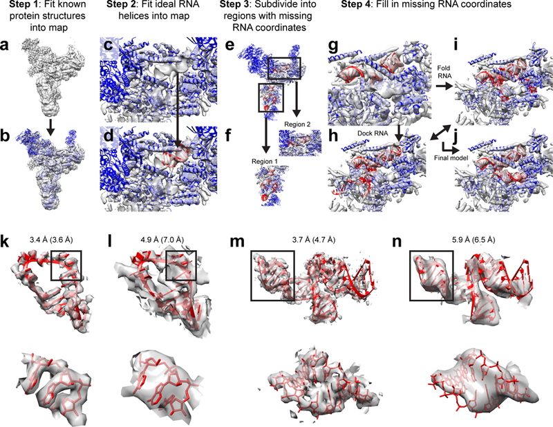
Figure 1.
The DRRAFTER framework. (a-j) Overview of the DRRAFTER pipeline: (a) Starting from a cryoEM density map (here the 5.9 u00c5 spliceosomal tri-snRNP map [ 9 ], gray), (b) individual protein structures (...
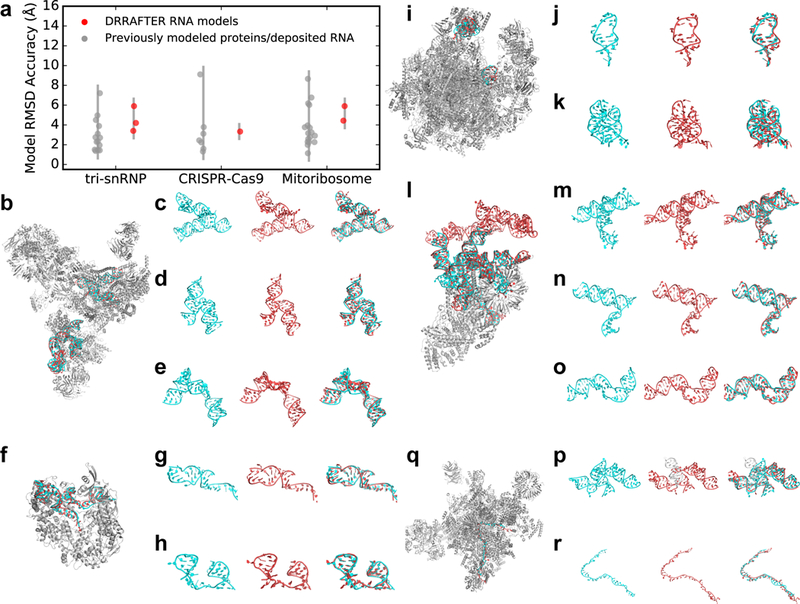
Figure 2.
DRRAFTER recovers near-native models over a diverse benchmark set and two blind test cases. (a) RMSDs of DRRAFTER models (red; each region modeled is plotted as a separate point) and previously modele...
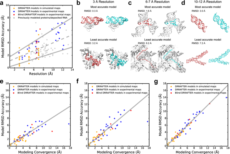
Figure 3.
Estimating DRRAFTER model accuracy. (a) RMSD accuracy versus local map resolution ( Supplementary Table 1 and Supplementary Table 3 ) for DRRAFTER models built into high- and low-resolution simulated ...

Figure 4.
DRRAFTER can accelerate manual model building into low-resolution density maps. Overlay of ten best scoring DRRAFTER models (RNA colored red, protein colored gray, density map colored transparent ligh...
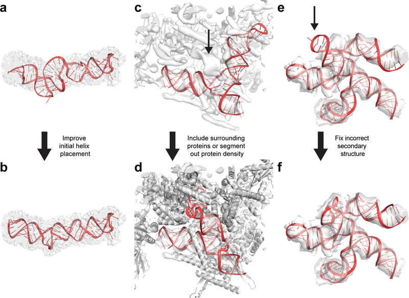
Figure 5.
Typical mistakes that may occur during DRRAFTER modeling and possible solutions. (a) Poor initial helix placement can lead to distorted final models, as shown here for residues 153u2013227 of the pack...
Figure images are served from the NIH/NLM PubMed Central Open Access Subset or Europe PMC; copyright remains with the publishers and authors.
💬 Discussion
0 commentsNo comments yet. Be the first to start a discussion!
Leave a Comment