Abstract
AbstractWe present a deep learning framework based on a generative adversarial network (GAN) to perform super-resolution in coherent imaging systems. We demonstrate that this framework can enhance the resolution of both pixel size-limited and diffraction-limited coherent imaging systems. The capabilities of this approach are experimentally validated by super-resolving complex-valued images acquired using a lensfree on-chip holographic microscope, the resolution of which was pixel size-limited. Using the same GAN-based approach, we also improved the resolution of a lens-based holographic imaging system that was limited in resolution by the numerical aperture of its objective lens. This deep learning-based super-resolution framework can be broadly applied to enhance the space-bandwidth product of coherent imaging systems using image data and convolutional neural networks, and provides a rapid, non-iterative method for solving inverse image reconstruction or enhancement problems in optics.
🔬 Techniques
💻 Software
✨ Fluorophores
🧪 Sample Preparation
🏭 Microscope Brands
🧪 Reagent Suppliers
📷 Detectors
🔎 Objectives
💻 Software Details
🏛️ Research Organizations (ROR)
Affiliated research institutions:
📋 Methods
First, we briefly summarize the methods that we have used in this paper; sub-sequent subsections will provide more information on specific methods employed in our work. We applied the presented deep learning-based super-resolution approach to two separate in-line holographic imaging systems to demonstrate the efficacy of the technique. As illustrated in Fig. 1a,b , the two implemented configurations were a pixel size-limited system (to be referred to as System A) and a diffraction-limited coherent microscopy system (to be referred to as System B). Despite using different methods to create the super-resolved images, as a result of the different image formation models, both of these systems followed similar general hologram reconstruction steps: (1) Raw holograms were collected at different sample to sensor distances, (2) Autofocus was used to determine the accurate sample to sensor distances, (3) Phase was recovered using a multi-height phase recovery algorithm. These steps will be detailed in the following subsections within the Methods 5 , 7 , 33 – 36 . Figure 1 Schematic of the coherent imaging systems. ( a ) A Lens-free on-chip holographic microscope. The sample is placed at a short distance (z 2 < 2 mm) above the image sensor chip. The resolution of this lensless on-chip imaging modality (without the use of additional degrees of freedom) is pixel size-limited due to its unit magnification. ( b ) A lens-based in-line holographic microscope, implemented by removing the condenser and switching the illumination to a partially-coherent light source on a conventional bright-field microscope. The resolution in this case is limited by the NA of the objective lens. For the pixel-super-resolution network (System A), the network training process is demonstrated in Fig. 2 , which summarizes both the hologram reconstruction procedure as well as the image super-resolving technique with and without using the network. The real and imaginary components of the phase recovered image pairs were used to train the network. Figure 2 Schematic of the training process for deep-learning based pixel super-resolution. An outline of the data required to generate the network input and ground truth images is shown, together with an overview of how both the traditional super-resolution is performed and how the deep learning super-resolution network is trained. For the diffraction-limited super-resolution network (System B), the network training process was demonstrated in Fig. 3 . In this case only the phase channel was used to train the network. Figure 3 Schematic of the training process for deep learning-based optical super-resolution for an NA-limited coherent imaging system. An outline of the data required to generate the network input and ground truth images is shown, together with an overview of how the deep learning super-resolution network is trained.
Show full methods section
First, we briefly summarize the methods that we have used in this paper; sub-sequent subsections will provide more information on specific methods employed in our work. We applied the presented deep learning-based super-resolution approach to two separate in-line holographic imaging systems to demonstrate the efficacy of the technique. As illustrated in Fig. 1a,b , the two implemented configurations were a pixel size-limited system (to be referred to as System A) and a diffraction-limited coherent microscopy system (to be referred to as System B). Despite using different methods to create the super-resolved images, as a result of the different image formation models, both of these systems followed similar general hologram reconstruction steps: (1) Raw holograms were collected at different sample to sensor distances, (2) Autofocus was used to determine the accurate sample to sensor distances, (3) Phase was recovered using a multi-height phase recovery algorithm. These steps will be detailed in the following subsections within the Methods 5 , 7 , 33 – 36 . Figure 1 Schematic of the coherent imaging systems. ( a ) A Lens-free on-chip holographic microscope. The sample is placed at a short distance (z 2 < 2 mm) above the image sensor chip. The resolution of this lensless on-chip imaging modality (without the use of additional degrees of freedom) is pixel size-limited due to its unit magnification. ( b ) A lens-based in-line holographic microscope, implemented by removing the condenser and switching the illumination to a partially-coherent light source on a conventional bright-field microscope. The resolution in this case is limited by the NA of the objective lens. For the pixel-super-resolution network (System A), the network training process is demonstrated in Fig. 2 , which summarizes both the hologram reconstruction procedure as well as the image super-resolving technique with and without using the network. The real and imaginary components of the phase recovered image pairs were used to train the network. Figure 2 Schematic of the training process for deep-learning based pixel super-resolution. An outline of the data required to generate the network input and ground truth images is shown, together with an overview of how both the traditional super-resolution is performed and how the deep learning super-resolution network is trained. For the diffraction-limited super-resolution network (System B), the network training process was demonstrated in Fig. 3 . In this case only the phase channel was used to train the network. Figure 3 Schematic of the training process for deep learning-based optical super-resolution for an NA-limited coherent imaging system. An outline of the data required to generate the network input and ground truth images is shown, together with an overview of how the deep learning super-resolution network is trained.
Generation of network input and ground truth super-resolved image labels
For the pixel size-limited coherent imaging system (System A), the super-resolved images were created by collecting multiple low-resolution holograms at different lateral positions, where the CMOS image sensor was sub-pixel shifted by a mechanical stage (MAX606, Thorlabs Inc., Newton, NJ, USA) to create a shift table. Once an accurate shift table was estimated, a shift-and-add based pixel super-resolution algorithm 33 was applied. The set-up used an illumination wavelength of 550 nm with a bandwidth (Δ λ ) of ~2 nm (WhiteLase Micro with acousto-optic tunable filter, NKT Photonics, Denmark), a single mode fiber (QPMJ-3S2.5A-488-3.5/125-1-0.3-1, OZ Optics, Canada) with a core diameter of ~3.5 μm and a source-to-sample distance ( z 1 ) of ~5 cm. As a result, the effective spatial coherence diameter at the sensor plane was larger than the width of the CMOS imager chip used in our on-chip imaging system. Therefore, the achievable resolution is limited by the temporal coherence length of the illumination 37 , which is defined as: 1 documentclass[12pt]{minimal} usepackage{amsmath} usepackage{wasysym} usepackage{amsfonts} usepackage{amssymb} usepackage{amsbsy} usepackage{mathrsfs} usepackage{upgreek} setlength{oddsidemargin}{-69pt} begin{document}$${rm{Delta }}{{L}}_{c}approx sqrt{frac{2,mathrm{ln},2}{pi }}cdot frac{{lambda }^{2}}{n{rm{Delta }}lambda }={rm{100.47}},mu {rm{m}}$$end{document} Δ L c ≈ 2 ln 2 π ⋅ λ 2 n Δ λ = 100.47 μ m where n = 1 is the refractive index. Assuming a sample-to-sensor distance ( z 2 ) of ~300 μm, the effective numerical aperture (NA) of the set-up was limited by the temporal coherence of the source, and is estimated to be: 2 documentclass[12pt]{minimal} usepackage{amsmath} usepackage{wasysym} usepackage{amsfonts} usepackage{amssymb} usepackage{amsbsy} usepackage{mathrsfs} usepackage{upgreek} setlength{oddsidemargin}{-69pt} begin{document}$${rm{NA}}=n,sin ,theta =nsqrt{1-{cos }^{2}theta }=nsqrt{1-{(frac{{z}_{2}}{{z}_{2}+{rm{Delta }}{L}_{c}})}^{2}}approx 0.6624$$end{document} NA = n sin θ = n 1 − cos 2 θ = n 1 − ( z 2 z 2 + Δ L c ) 2 ≈ 0.6624 Based on this effective numerical aperture and ignoring the pixel size at the hologram plane, the achievable coherence-limited resolution of our on-chip microscope is approximated as 4 : 3 documentclass[12pt]{minimal} usepackage{amsmath} usepackage{wasysym} usepackage{amsfonts} usepackage{amssymb} usepackage{amsbsy} usepackage{mathrsfs} usepackage{upgreek} setlength{oddsidemargin}{-69pt} begin{document}$$dpropto frac{lambda }{{rm{N}}{rm{A}}}=frac{0.55}{0.6624}={rm{0.8303}},mu {rm{m}}$$end{document} d ∝ λ N A = 0.55 0.6624 = 0.8303 μ m At the hologram/detector plane, however, the effective pixel pitch of the CMOS image sensor (IMX 081 RGB sensor, Sony Corp., Minato, Tokyo, Japan, pixel size of 1.12 μm) using only one color channel is 2.24 μm. Based on this, the effective pixel size for each super-resolved image after the application of the pixel super-resolution algorithm to 4 raw holograms (2 × 2 lateral positions), 9 raw holograms (3 × 3 lateral positions), and 36 raw holograms (6 × 6 lateral positions) are 1.12 μm, 0.7467 μm and 0.3733 μm, respectively. Based on eq. ( 3 ), the effective pixel size achieved by pixel super-resolution using 6 × 6 lateral positions can adequately sample the specimen’s holographic diffraction pattern and is limited by temporal coherence. All of the other images (using 1 × 1, 2 × 2 and 3 × 3 raw holograms) remain pixel-limited in their achievable spatial resolution. This pixel-limited resolution of an on-chip holographic microscope is a result of its unit magnification. This allows the imaging system to have a large imaging field-of-view (FOV) that is only limited by the active area of the opto-electronic image sensor chip. This can easily reach 20–30 mm 2 and > 10 cm 2 using state-of-the-art CMOS and CCD imagers, respectively 5 . For the second set-up (System B), which used lens-based holographic imaging for diffraction-limited coherent microscopy, the low- and high-resolution images were acquired with different objective lenses. For this set-up, the illumination was performed using a fiber coupled laser diode with an illumination wavelength of 532 nm. A 4×/0.13 NA objective lens was used to acquire lower resolution images, achieving a diffraction limited resolution of ~4.09 µm and an effective pixel size of ~1.625 µm. A 10×/0.30 NA objective lens was used to acquire the higher resolution images (ground truth labels), achieving a resolution of 1.773 µm and an effective pixel size of ~0.65 µm. Autofocusing and singular value decomposition-based background subtraction For both types of coherent imaging systems, holograms at 8 different sample-to-sensor distances were collected to perform the multi-height phase recovery 5 , 7 , 33 – 36 . This algorithm requires accurate knowledge of the sample-to-sensor distances used. These were estimated using an autofocusing algorithm. The autofocusing algorithm assigned zero phase to the raw holograms collected by the image sensor and propagated them to different sample to sensor heights using the free space angular spectrum approach 4 . The Tamura of the gradient (ToG) edge sparsity-based criterion was computed 38 at each height for each hologram and used to determine the corresponding refocusing distance. For the lens-based diffraction-limited coherent imaging system (System B), the autofocusing algorithm required an additional background subtraction step. For undesired particles or dust associated with the objective lens or other parts of the optical microscope, the diffraction pattern that is formed is independent of the sample and its position. Using this information, a singular value decomposition (SVD)-based background subtraction was performed 39 , after which the ToG-based autofocusing algorithm was successfully applied. Multi-height phase recovery The iterative multi-height phase recovery technique 34 was applied to eliminate the holographic image artifacts (twin image and self-interference terms 4 ) in both of the coherent imaging systems that were used in this work. To perform this, an initial zero-phase was assigned to the intensity/amplitude measurement at the 1st hologram height. Next, the iterative algorithm begins by propagating the complex field to each hologram height until the 8 th height is reached, and then backpropagates the resulting fields until the 1 st height is reached. While the phase was retained at each hologram height, the amplitude was updated by averaging current amplitude and the square root of the measured intensity at each height. Registration between lower resolution and higher resolution (ground truth) images Image registration plays a key role in generating the training and testing image pairs for the network in both the pixel size-limited and diffraction-limited coherent imaging systems. A pixel-wise registration must be performed to ensure the success of the network in learning the transformation to perform super-resolution. For both super resolution methods, the low-resolution input images were initially bicubically up-sampled. Following this, a correlation-based registration, which corrected any rotational misalignments or shifts between the images was performed. This registration process correlated the spatial patterns of the phase images and used the correlation to establish an affine transform matrix. This was in turn be applied to the high-resolution images to ensure proper matching of the corresponding fields-of-view between the low-resolution images and their corresponding ground truth labels. Finally, each image was cropped by 50 pixels to each side to accommodate for any relative shift that may have occurred. For the diffraction-limited coherent imaging system (System B), an additional rough FOV matching step was required before the registration above. For this step, the higher resolution phase images was first stitched together, by calculating the overlap between neighboring images, and using this to stitch them together into a larger image. The corresponding lower resolution phase images are then matched to this larger image. This is done by creating a correlation score matrix between the stitched high resolution image and each of the lower resolution images. Whichever portion of the matrix has the highest correlation score is used to determine which portion of the fused image is cropped out and is used as the input for the network. GAN architecture and training process Once the high and low resolution image pairs were accurately registered, they were cropped into smaller image patches (128 × 128 pixels), which were used to train the network. The architectures of the generator ( G ) and the discriminator ( D ) that make up the GAN can be seen in Fig. 4 . For both the pixel-size limited and the diffraction-limited coherent imaging systems, the discriminator loss function is defined as: 4 documentclass[12pt]{minimal} usepackage{amsmath} usepackage{wasysym} usepackage{amsfonts} usepackage{amssymb} usepackage{amsbsy} usepackage{mathrsfs} usepackage{upgreek} setlength{oddsidemargin}{-69pt} begin{document}$${l}_{{rm{d}}{rm{i}}{rm{s}}{rm{c}}{rm{r}}{rm{i}}{rm{m}}{rm{i}}{rm{n}}{rm{a}}{rm{t}}{rm{o}}{rm{r}}}=D{(G({x}_{{rm{i}}{rm{n}}{rm{p}}{rm{u}}{rm{t}}}))}^{2}+{(1-D({z}_{{rm{l}}{rm{a}}{rm{b}}{rm{e}}{rm{l}}}))}^{2}$$end{document} l d i s c r i m i n a t o r = D ( G ( x i n p u t ) ) 2 + ( 1 − D ( z l a b e l ) ) 2 where D (.) and G (.) refer to the discriminator and generator network operators, respectively, x input is the lower resolution input to the generator, and z label is the higher resolution label image. For the lensfree holographic imaging system (System A), the generator loss function was defined by: 5 documentclass[12pt]{minimal} usepackage{amsmath} usepackage{wasysym} usepackage{amsfonts} usepackage{amssymb} usepackage{amsbsy} usepackage{mathrsfs} usepackage{upgreek} setlength{oddsidemargin}{-69pt} begin{document}$${l}_{{rm{g}}{rm{e}}{rm{n}}{rm{e}}{rm{r}}{rm{a}}{rm{t}}{rm{o}}{rm{r}}}={L}_{1}{{z}_{{rm{l}}{rm{a}}{rm{b}}{rm{e}}{rm{l}}},G({x}_{{rm{i}}{rm{n}}{rm{p}}{rm{u}}{rm{t}}})}+gamma times TV{G({x}_{{rm{i}}{rm{n}}{rm{p}}{rm{u}}{rm{t}}})}+alpha times {(1-D(G({x}_{{rm{i}}{rm{n}}{rm{p}}{rm{u}}{rm{t}}})))}^{2}$$end{document} l g e n e r a t o r = L 1 { z l a b e l , G ( x i n p u t ) } + γ × T V { G ( x i n p u t ) } + α × ( 1 − D ( G ( x i n p u t ) ) ) 2 Figure 4 Diagram of the GAN structure. ( a ) Structure of the generator portion of the network. ( b ) Structure of the discriminator portion of the network. The L 1 { z label , G ( x input )} term is calculated using: 6 documentclass[12pt]{minimal} usepackage{amsmath} usepackage{wasysym} usepackage{amsfonts} usepackage{amssymb} usepackage{amsbsy} usepackage{mathrsfs} usepackage{upgreek} setlength{oddsidemargin}{-69pt} begin{document}$${L}_{1}{{z}_{{rm{label}}},G({x}_{{rm{input}}})}={{rm{E}}}_{n_mathrm{pixels}}({{rm{E}}}_{n_mathrm{channels}}(|G({x}_{{rm{input}}})-{z}_{{rm{label}}}|))$$end{document} L 1 { z label , G ( x input ) } = E n _ pixels ( E n _ channels ( | G ( x input ) − z label | ) ) This finds the absolute difference between each pixel of the generator output image and its corresponding label. E n_pixels (.) and E n_channels (.) are the expectation values for the pixels with in each image and the channels of each image, respectively. TV { G ( x input )} represents the total variation loss, which acts as a regularization term, applied to the generator output. Total variation ( TV ) is defined as: 7 documentclass[12pt]{minimal} usepackage{amsmath} usepackage{wasysym} usepackage{amsfonts} usepackage{amssymb} usepackage{amsbsy} usepackage{mathrsfs} usepackage{upgreek} setlength{oddsidemargin}{-69pt} begin{document}$$TV={E}_{n_mathrm{channels}}({sum }_{i,j}|G{({x}_{{rm{input}}})}_{i+1,j}-G{({x}_{{rm{input}}})}_{i,j}|+|G{({x}_{{rm{input}}})}_{i,j+1}-G{({x}_{{rm{input}}})}_{i,j}|)$$end{document} T V = E n _ channels ( ∑ i , j | G ( x input ) i + 1 , j − G ( x input ) i , j | + | G ( x input ) i , j + 1 − G ( x input ) i , j | ) where the i and j indices represent the location of the pixels within each channel of the image. The last term in eq. ( 5 ) (i.e., α × (1 − D (G( x input ))) 2 ) is a function of how well the output image of the generator network can be predicted by the discriminator network. α and γ are regularization parameters which were set to 0.00275 and 0.015 respectively. As a result of these parameters, the L 1 loss term, L 1 { z label , G ( x input )}, made up 60% of the overall loss, while the total variation term, γ × TV { G ( x input )}, was approximately 0.25% of the total loss. The discriminator loss term, α × (1 − D ( G ( x input ))) 2 , made up the remainder of the overall generator loss. Once the networks were successfully trained, they reach a state of equilibrium where the discriminator network cannot successfully discriminate between the output and label images, and D ( G ( x input )) converged to approximately 0.5. The loss function for the lens-based coherent microscope images (System B) incorporated an additional structural similarity index (SSIM) 32 term in addition to the terms included for the lensfree on-chip imaging system, i.e.: 8 documentclass[12pt]{minimal} usepackage{amsmath} usepackage{wasysym} usepackage{amsfonts} usepackage{amssymb} usepackage{amsbsy} usepackage{mathrsfs} usepackage{upgreek} setlength{oddsidemargin}{-69pt} begin{document}$${l}_{{rm{g}}{rm{e}}{rm{n}}{rm{e}}{rm{r}}{rm{a}}{rm{t}}{rm{o}}{rm{r}}}={L}_{1}{{z}_{{rm{l}}{rm{a}}{rm{b}}{rm{e}}{rm{l}}},G({x}_{{rm{i}}{rm{n}}{rm{p}}{rm{u}}{rm{t}}})}+gamma times TV{G({x}_{{rm{i}}{rm{n}}{rm{p}}{rm{u}}{rm{t}}})}+alpha times {(1-D(G({x}_{{rm{i}}{rm{n}}{rm{p}}{rm{u}}{rm{t}}})))}^{2},+beta times {rm{S}}{rm{S}}{rm{I}}{rm{M}}{G({x}_{{rm{i}}{rm{n}}{rm{p}}{rm{u}}{rm{t}}}),{z}_{{rm{l}}{rm{a}}{rm{b}}{rm{e}}{rm{l}}}}$$end{document} l g e n e r a t o r = L 1 { z l a b e l , G ( x i n p u t ) } + γ × T V { G ( x i n p u t ) } + α × ( 1 − D ( G ( x i n p u t ) ) ) 2 + β × S S I M { G ( x i n p u t ) , z l a b e l } β is a regularization parameter, set to 0.01, and SSIM{ x , z } is defined as 32 : 9 documentclass[12pt]{minimal} usepackage{amsmath} usepackage{wasysym} usepackage{amsfonts} usepackage{amssymb} usepackage{amsbsy} usepackage{mathrsfs} usepackage{upgreek} setlength{oddsidemargin}{-69pt} begin{document}$${rm{SSIM}}(x,z)=frac{(2{mu }_{x}{mu }_{z}+{c}_{1})(2{sigma }_{x,z}+{c}_{2})}{({mu }_{x}^{2}+{mu }_{z}^{2}+{c}_{1})({sigma }_{x}^{2}+{sigma }_{z}^{2}+{c}_{2})}$$end{document} SSIM ( x , z ) = ( 2 μ x μ z + c 1 ) ( 2 σ x , z + c 2 ) ( μ x 2 + μ z 2 + c 1 ) ( σ x 2 + σ z 2 + c 2 ) where μ x , μ z are the averages of x , z ; documentclass[12pt]{minimal} usepackage{amsmath} usepackage{wasysym} usepackage{amsfonts} usepackage{amssymb} usepackage{amsbsy} usepackage{mathrsfs} usepackage{upgreek} setlength{oddsidemargin}{-69pt} begin{document}$${sigma }_{x}^{2},,{sigma }_{z}^{2}$$end{document} σ x 2 , σ z 2 are the variances of x , z , respectively; σ x,z is the covariance of x and z ; and c 1 , c 2 are dummy variables used to stabilize the division with a small denominator. The term β × SSIM{ G ( x input ), z label } was set to make up ~15% of the total generator loss, with the rest of the regularization weights reduced in value accordingly. Our generator network used an adapted U-net architecture 40 . The network began with a convolutional layer that increased the number of channels to 32 and a leaky rectified linear (LReLU) unit, defined as: 10 documentclass[12pt]{minimal} usepackage{amsmath} usepackage{wasysym} usepackage{amsfonts} usepackage{amssymb} usepackage{amsbsy} usepackage{mathrsfs} usepackage{upgreek} setlength{oddsidemargin}{-69pt} begin{document}$${rm{L}}{rm{R}}{rm{e}}{rm{L}}{rm{U}},(x)={begin{array}{ll}x & {rm{for}},x > 0\ 0.1x & {rm{otherwise}}end{array}$$end{document} L R e L U ( x ) = { x for x > 0 0.1 x otherwise Following this layer, there was a down-sampling and an up-sampling section. Each section consists of three distinct layers, each made up of separate convolution blocks (see Fig. 4a ). For the down-sampling section, these residual blocks consisted of two convolution layers with LReLU units acting upon them. At the output of the second convolution of each block the number of channels was doubled. The down-sampling blocks were connected by an average-pooling layer of stride two that down-samples the output of the previous block by a factor of two in both lateral dimensions (see Fig. 4a ). The up-sampling section of the network used a reverse structure to reduce the number of channels and return each channel to its original size. Similar to the down sampling section, each block contained two convolutional layers, each activated by a LReLU layer. At the input of each block, the previous output was up-sampled using a bilinear interpolation and concatenated with the output of the down-sampling path at the same level (see Fig. 4a ). Between the two paths, convolutional layer was added to maintain the number of the feature maps from the output of the last residual block to the beginning of the down-sampling path (Fig. 4a ). Finally, a convolutional layer was used to reduce the number of output channels to match the size of the label. The discriminator portion of the network was made up of a convolutional layer, followed by five discriminator blocks, an average pooling layer and two fully connected layers which reduced the output to a single value (see Fig. 4b ). Both the label images and the output of the generator network were input into the initial convolutional layer discriminator network. This layer was used to increase the number of channels to 32 and was followed by five discriminator blocks all containing two convolutional layers activated upon by LReLU functions. The first convolution was used to maintain the size of the output, and the second doubled the number of channels while halving the size of the output in each lateral dimension. Next, the average pooling layer was used to find the mean of each channel, reducing the dimensionality to a vector of length 1024 for each patch. Each of these vectors were subsequently fed into two fully connected layers and LReLU activation layers in series. While the first fully connected layer did not change the dimensionality, the second reduced the output of each patch to a single number which was in turn input into a sigmoid function. The output of the sigmoid function represents the probability of the input being either real or fake and was used as part of the generator’s loss function. The filter size for each convolution was set to be 3 × 3. The trainable parameters are updated using an adaptive moment estimation (Adam) 41 optimizer with a learning rate 1 × 10 −4 for the generator network and 1 × 10 −5 for the discriminator network. The image data were augmented by randomly flipping 50% of the images, and randomly choosing a rotation angle (0, 90, 180, 270 degrees). For each iteration that the discriminator is updated, the generator network is updated four times, which helps the discriminator avoid overfitting to the target images. The convolutional layer weights are initialized using a truncated normal distribution while the network bias terms are initialized to zero. A batch size of 10 is used for the training, and a batch size of 25 is used for validation. The networks chosen for blind testing were those with the lowest validation loss. The number of training steps as well as the training time for each network are reported in Table 1 , and the testing times are reported in Table 2 . Table 1 Training details for the deep neural networks. Resolution limiting factor Tissue type Low resolution input type Training dataset size (number of patches before augmentation) Training time (s) Number of iterations Pixel size-limited (System A) Pap smear 1 × 1 raw hologram 56250 9,078 17,000 Lung 1 × 1 raw hologram 83700 17,052 28,000 Lung 2 × 2 raw holograms 83700 9,363 15,000 Lung 3 × 3 raw holograms 83700 30,480 52,500 Diffraction-limited (System B) Pap smear 4×/0.13 NA objective lens 65475 46,411 100,000 All the networks were trained with a batch size of 10 using 128 × 128 pixel patches. Table 2 Time for each network to output a 1940 × 1940 pixel image. Resolution limiting factor Tissue type Low resolution input type Testing Time (s/image) Pixel size-limited (System A) Pap smear 1 × 1 raw hologram 1.42 Lung 1 × 1 raw hologram 1.37 Lung 2 × 2 raw holograms 1.38 Lung 3 × 3 raw holograms 1.38 Diffraction-limited (System B) Pap smear 4×/0.13 NA objective lens 1.26 Each measurement is the average time, calculated using 150 test images.
Software implementation details
The network was developed using a desktop computer running the Windows 10 operating system. The desktop uses an Nvidia GTX 1080 Ti GPU, a Core i7-7900K CPU running at 3.3 GHz, and 64 GB of RAM. The network was programmed using Python (version 3.6.0) with the TensorFlow library (version 1.7.0).
Sample preparation De-identified
Pap smear slides were provided by the UCLA Department of Pathology (Institutional Review Board no. 11–003335) using ThinPrep® and SurePath TM preparation. De-identified Hematoxylin and Eosin (H&E) stained human lung tissue slides were acquired from the UCLA Translational Pathology Core Laboratory. We used existing and anonymous specimen, where no subject related information was linked or can be retrieved.
📊 Figures
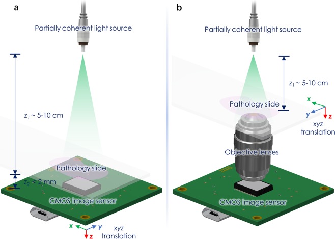
Figure 1
Schematic of the coherent imaging systems. ( a ) A Lens-free on-chip holographic microscope. The sample is placed at a short distance (z 2 <u20092u2009mm) above the image sensor chip. The resolutio...
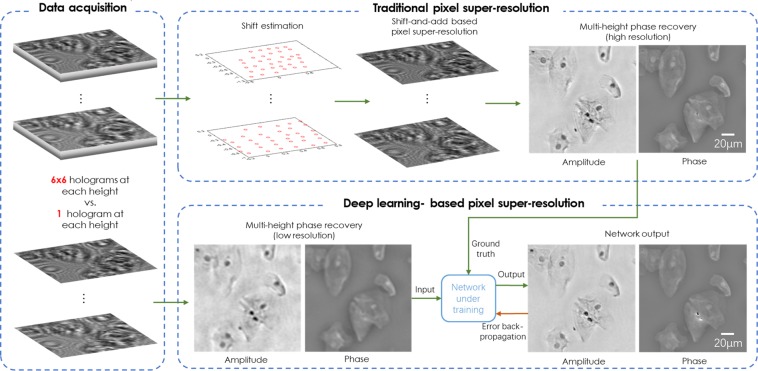
Figure 2
Schematic of the training process for deep-learning based pixel super-resolution. An outline of the data required to generate the network input and ground truth images is shown, together with an overv...
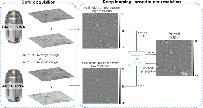
Figure 3
Schematic of the training process for deep learning-based optical super-resolution for an NA-limited coherent imaging system. An outline of the data required to generate the network input and ground t...
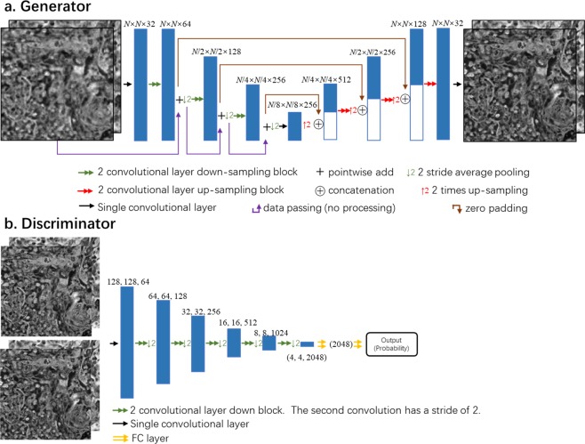
Figure 4
Diagram of the GAN structure. ( a ) Structure of the generator portion of the network. ( b ) Structure of the discriminator portion of the network.
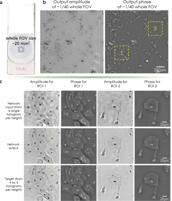
Figure 5
Visualized result for the pixel size-limited system. Deep learning-based pixel super-resolution imaging of a Pap smear slide under 550u2009nm illumination. ( a ) Whole FOV of the lensfree imaging syst...
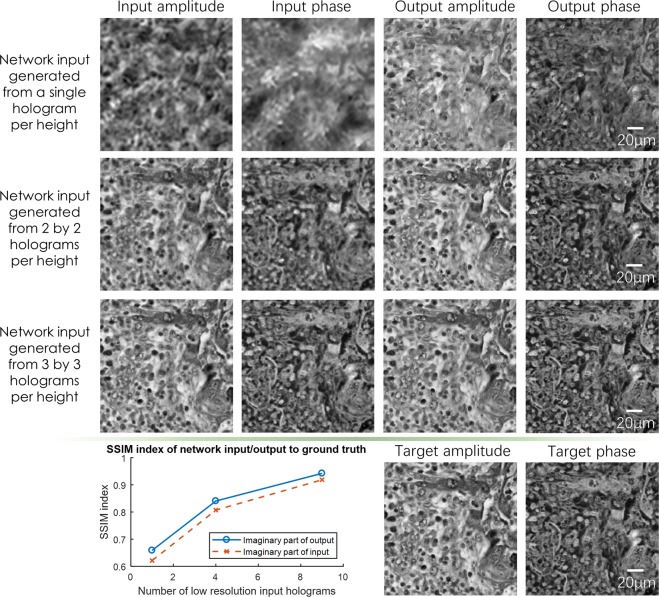
Figure 6
Visualized result for the pixel size-limited system. Comparison of the performances for the deep-learning-based pixel super-resolution methods using different input images. The sample is a Massonu2019...
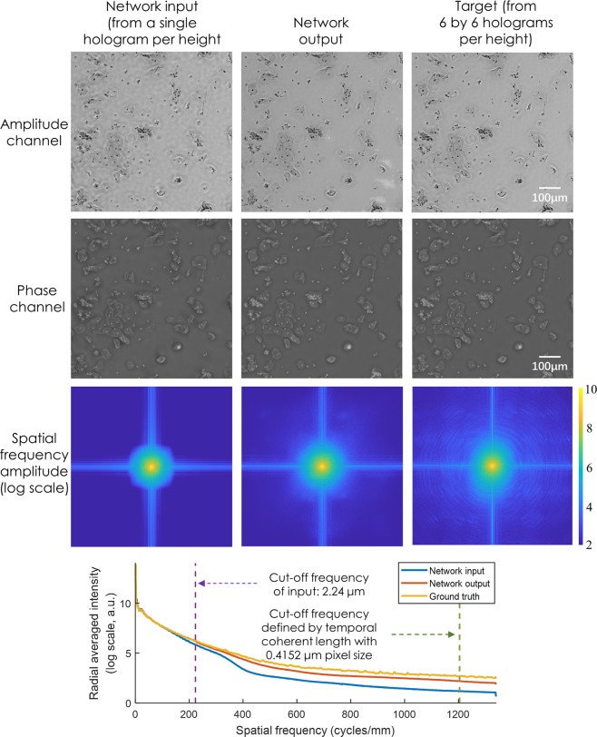
Figure 7
Spatial frequency analysis for the pixel size-limited system. Radially-averaged spatial frequency spectra of the network input, network output and target images, corresponding to a lensfree on-chip co...
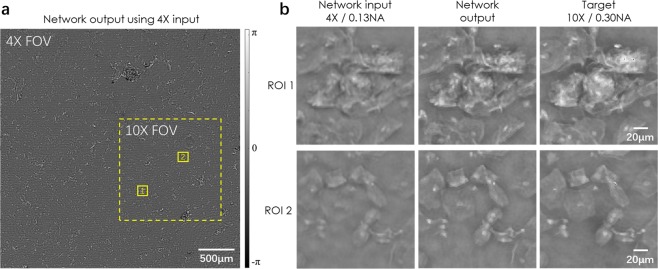
Figure 8
Visualized result for the diffraction-limited system. Deep learning-based super-resolution imaging of a Pap smear slide under 532u2009nm illumination using a lens-based holographic microscope. ( a ) P...
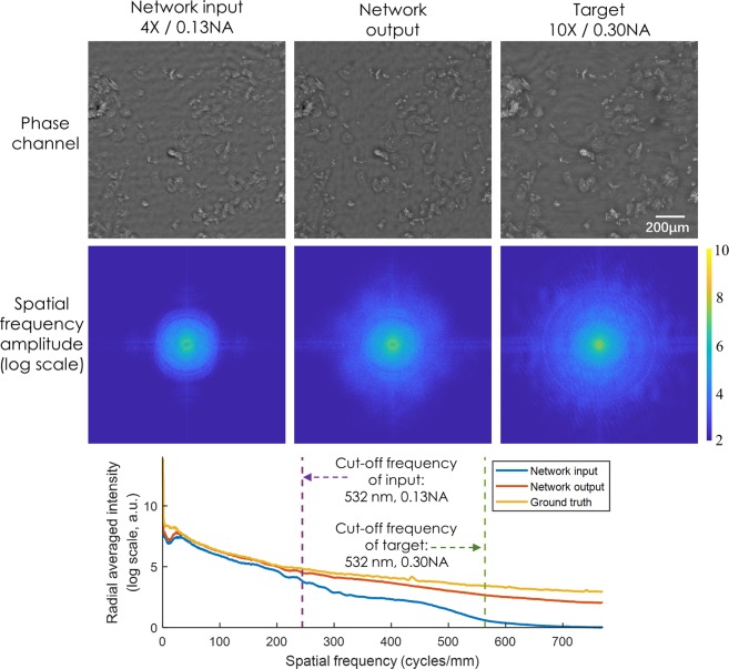
Figure 9
Spatial frequency analysis for the diffraction-limited system. Radially-averaged spatial frequency spectra of the network input, network output and target images, corresponding to a lens-based coheren...
Figure images are served from the NIH/NLM PubMed Central Open Access Subset or Europe PMC; copyright remains with the publishers and authors.
💬 Discussion
0 commentsNo comments yet. Be the first to start a discussion!
Leave a Comment