Abstract
AbstractCurrent liver fibrosis scoring by computer-assisted image analytics is not fully automated as it requires manual preprocessing (segmentation and feature extraction) typically based on domain knowledge in liver pathology. Deep learning-based algorithms can potentially classify these images without the need for preprocessing through learning from a large dataset of images. We investigated the performance of classification models built using a deep learning-based algorithm pre-trained using multiple sources of images to score liver fibrosis and compared them against conventional non-deep learning-based algorithms - artificial neural networks (ANN), multinomial logistic regression (MLR), support vector machines (SVM) and random forests (RF). Automated feature classification and fibrosis scoring were achieved by using a transfer learning-based deep learning network, AlexNet-Convolutional Neural Networks (CNN), with balanced area under receiver operating characteristic (AUROC) values of up to 0.85–0.95 versus ANN (AUROC of up to 0.87–1.00), MLR (AUROC of up to 0.73–1.00), SVM (AUROC of up to 0.69–0.99) and RF (AUROC of up to 0.94–0.99). Results indicate that a deep learning-based algorithm with transfer learning enables the construction of a fully automated and accurate prediction model for scoring liver fibrosis stages that is comparable to other conventional non-deep learning-based algorithms that are not fully automated.
🔬 Techniques
🧪 Sample Preparation
🏭 Microscope Brands
🧪 Reagent Suppliers
💻 Software Details
🏛️ Research Organizations (ROR)
Affiliated research institutions:
📋 Methods
Tissue preparation Male
Wistar rats (average weight of 220 g) were housed 2 per cage in the Biological Resource Centre (BRC) of Biopolis, Agency for Science, Technology and Research (A*STAR) with free access to laboratory chow and water in a 12:12 h light/dark schedule. The Institutional Animal Care and Use Committee (IACUC, Biological Resource Centre, A*STAR) approved all animal-related experiments and all methods were performed in accordance with the relevant guidelines and regulations. A total of 25 rats were randomly separated into a group of 21 for thioacetamide (TAA) treatment, and a group of 4 as controls. The 21 rats in the TAA-treated group were sacrificed at time-points of 4, 6, 7, 8, 10 and 12 weeks. Another 4 rats in the control group were sacrificed at week 0 without treatment. Cardiac perfusion with 4% paraformaldehyde was performed to flush out blood cells and the liver was fixed before harvesting. Collagen staining and pathological scoring 4 biopsy samples were taken from each rat liver. They were formalin-fixed, paraffin-embedded, cut into 5 µm sections and stained for histological assessment. A total of 100 slides from 25 paraffin blocks were stained with Sirius Red (SR) stain kit (Picro Sirius Red Stain Kit, ab150681, Abcam). Each SR-stained sample was blinded and scored by a pathologist to reduce any bias using the Metavir scoring system 7 . In the Metavir system, liver fibrosis was classified into five stages from F0 to F4 according to the severity of fibrosis: no fibrosis, fibrous portal expansion, few bridges or septa, numerous bridges or septa, and cirrhosis 18 . The number of samples that were categorized into each stage was: 20 F0, 20 F1, 20 F2, 20 F3 and 20 F4. Image acquisition Another 4 paired biopsy samples were taken from the previously processed 25 paraffin blocks for imaging using Second Harmonic Generation (SHG) microscopy. A total of 100 paired slides from 25 paraffin blocks were used and SHG images were acquired using the Olympus IX81 system. The laser was tuned to 810 nm to excite the samples and SHG signals were recorded at 405 nm using a 20X objective lens. A nine-by-seven multi-tile image was acquired for every slide with a final image size of 12 mm 2 (4 × 3 mm).
Show full methods section
Tissue preparation Male
Wistar rats (average weight of 220 g) were housed 2 per cage in the Biological Resource Centre (BRC) of Biopolis, Agency for Science, Technology and Research (A*STAR) with free access to laboratory chow and water in a 12:12 h light/dark schedule. The Institutional Animal Care and Use Committee (IACUC, Biological Resource Centre, A*STAR) approved all animal-related experiments and all methods were performed in accordance with the relevant guidelines and regulations. A total of 25 rats were randomly separated into a group of 21 for thioacetamide (TAA) treatment, and a group of 4 as controls. The 21 rats in the TAA-treated group were sacrificed at time-points of 4, 6, 7, 8, 10 and 12 weeks. Another 4 rats in the control group were sacrificed at week 0 without treatment. Cardiac perfusion with 4% paraformaldehyde was performed to flush out blood cells and the liver was fixed before harvesting. Collagen staining and pathological scoring 4 biopsy samples were taken from each rat liver. They were formalin-fixed, paraffin-embedded, cut into 5 µm sections and stained for histological assessment. A total of 100 slides from 25 paraffin blocks were stained with Sirius Red (SR) stain kit (Picro Sirius Red Stain Kit, ab150681, Abcam). Each SR-stained sample was blinded and scored by a pathologist to reduce any bias using the Metavir scoring system 7 . In the Metavir system, liver fibrosis was classified into five stages from F0 to F4 according to the severity of fibrosis: no fibrosis, fibrous portal expansion, few bridges or septa, numerous bridges or septa, and cirrhosis 18 . The number of samples that were categorized into each stage was: 20 F0, 20 F1, 20 F2, 20 F3 and 20 F4. Image acquisition Another 4 paired biopsy samples were taken from the previously processed 25 paraffin blocks for imaging using Second Harmonic Generation (SHG) microscopy. A total of 100 paired slides from 25 paraffin blocks were used and SHG images were acquired using the Olympus IX81 system. The laser was tuned to 810 nm to excite the samples and SHG signals were recorded at 405 nm using a 20X objective lens. A nine-by-seven multi-tile image was acquired for every slide with a final image size of 12 mm 2 (4 × 3 mm).
Image pre-processing for collagen content
All raw images acquired from SHG microscopy were imported into the MATLAB Image Processing Toolbox (Mathworks) for further processing. The resulting gray-scale images were first adjusted by contrast enhancement 19 and then transformed into binary images using adaptive-thresholding 9 – 11 . To fully reproduce the distribution of collagen fibers and eliminate any background signal, morphological closing was then performed to smooth the binary mask of the collagen and segments with less than 5 pixels were removed 9 – 11 . Feature extraction and quantification for collagen content Total collagen content and previously described collagen features, including collagen fiber morphology 20 , 21 and collagen fiber connectivity-related texture measurements 22 , were investigated. A total of 21 morphological features specific to tubular-shaped objects including length, width, orientation, cross-link spaces and cross-link density, etc. and 109 textural features of both gray-level co-occurrence matrix (GLCM) and transform-based pattern including contrast, correlation, average, variation, entropy etc. from the occurrence matrix and Fourier, Gabor, and wavelet transformation were extracted from the processed SHG images.
Model construction for deep learning-based algorithms
For deep learning, a pre-trained AlexNet-CNN network was used for training and testing purposes. This network was made up of 1 input layer, 7 hidden layers (5 convolution layers and 2 fully connected layers) and 1 output layer using batch stochastic gradient descent, with specific values for momentum and weight decay 17 . The input and output layers of the original AlexNet-CNN network were replaced accordingly for liver fibrosis assessment as previously reported 15 , 16 , where the processed SHG images were first resized and duplicated to 224 × 224 × 3 pixels to fit into the model as input images. There were 2 max pooling layers of size 2 × 2 pixels after the first and second convolution layer where the size and number of filters are 11 × 11 × 3 pixels, 96 and 5 × 5 × 96 pixels, 256, respectively. Another 3 convolution layers where the size and number of filters are 3 × 3 × 256 pixels, 384 and 3 × 3 × 384 pixels, 384 and 3 × 3 × 384 pixels, 256, respectively were also implemented before the third max pooling layer. Layers 6 and 7 are 4096-dimension fully connected layers where the input matrix is transformed into a vector for Softmax activation function through General MATRIX Vector Multiply (GEMV) approach. The final output layer contained 5 possible outcomes corresponding to the 5 liver fibrosis stages from F0 to F4 using the Metavir scoring. Model construction for non-deep learning-based algorithms ANN, MLR, SVM and RF-based algorithms were applied for the training and testing datasets with pre-processed images and selected features to test the sample classification. The leave-one-out cross validation rule was applied. For ANN, various combinations of layers and nodes a) 1 hidden layer with 10 nodes; b) 1 hidden layer with 20 nodes and c) 2 hidden layers with 20 nodes each and feed-forward neural network were established for the analysis using a back-propagation orientated gradient descent training approach to optimize the loss. For MLR, the coefficients of the predicted probability were calculated using the logistic function, g, the logit (log odds): documentclass[12pt]{minimal} usepackage{amsmath} usepackage{wasysym} usepackage{amsfonts} usepackage{amssymb} usepackage{amsbsy} usepackage{mathrsfs} usepackage{upgreek} setlength{oddsidemargin}{-69pt} begin{document}$${rm{g}}({rm{p}}({rm{x}}))=,mathrm{ln}(frac{p(x)}{1-p(x)})={beta }_{0}+{beta }_{1}{x}_{1}+ldots +{beta }_{n}{x}_{n}$$end{document} g ( p ( x ) ) = ln ( p ( x ) 1 − p ( x ) ) = β 0 + β 1 x 1 + … + β n x n The coefficients documentclass[12pt]{minimal} usepackage{amsmath} usepackage{wasysym} usepackage{amsfonts} usepackage{amssymb} usepackage{amsbsy} usepackage{mathrsfs} usepackage{upgreek} setlength{oddsidemargin}{-69pt} begin{document}$${beta }_{0}$$end{document} β 0 , documentclass[12pt]{minimal} usepackage{amsmath} usepackage{wasysym} usepackage{amsfonts} usepackage{amssymb} usepackage{amsbsy} usepackage{mathrsfs} usepackage{upgreek} setlength{oddsidemargin}{-69pt} begin{document}$${beta }_{1}$$end{document} β 1 , … documentclass[12pt]{minimal} usepackage{amsmath} usepackage{wasysym} usepackage{amsfonts} usepackage{amssymb} usepackage{amsbsy} usepackage{mathrsfs} usepackage{upgreek} setlength{oddsidemargin}{-69pt} begin{document}$${beta }_{n}$$end{document} β n were estimated with the maximum likelihood method. For SVM, a hyperplane was constructed for optimally and correctly classifying the images into fibrosis stages based on the feature values in the m-dimensional space. The radial basis function (RBF) kernel was used as the distance measurement between adjacent subject vectors documentclass[12pt]{minimal} usepackage{amsmath} usepackage{wasysym} usepackage{amsfonts} usepackage{amssymb} usepackage{amsbsy} usepackage{mathrsfs} usepackage{upgreek} setlength{oddsidemargin}{-69pt} begin{document}$${x}_{1}$$end{document} x 1 and documentclass[12pt]{minimal} usepackage{amsmath} usepackage{wasysym} usepackage{amsfonts} usepackage{amssymb} usepackage{amsbsy} usepackage{mathrsfs} usepackage{upgreek} setlength{oddsidemargin}{-69pt} begin{document}$${x}_{2}$$end{document} x 2 , i.e., documentclass[12pt]{minimal} usepackage{amsmath} usepackage{wasysym} usepackage{amsfonts} usepackage{amssymb} usepackage{amsbsy} usepackage{mathrsfs} usepackage{upgreek} setlength{oddsidemargin}{-69pt} begin{document}$${rm{K}}({x}_{1},{x}_{2})=exp (-frac{({x}_{1}-{{x}_{2})}^{2}}{2{sigma }^{2}})$$end{document} K ( x 1 , x 2 ) = exp ( − ( x 1 − x 2 ) 2 2 σ 2 ) documentclass[12pt]{minimal} usepackage{amsmath} usepackage{wasysym} usepackage{amsfonts} usepackage{amssymb} usepackage{amsbsy} usepackage{mathrsfs} usepackage{upgreek} setlength{oddsidemargin}{-69pt} begin{document}$$sigma $$end{document} σ controls the width of the kernel. For RF, the training algorithm applies the general techniques of bootstrap aggregating, or bagging, to trees learners where 100 decision tree bagging with random sample replacement was used to generate the classification results and the majority vote in the case of classification trees was used for final predictions. The core algorithm for building decision trees called ID3 by J. R. Quinlan employs a top-down, greedy search through the space of possible branches with no backtracking. ID3 uses Entropy and Information Gain to construct a decision tree 23 .
Statistical analysis Kruskal-Wallis
(KW) tests were used to assess the performance of various classification models for their prediction capabilities in SPSS (IBM Corporation). Post-hoc analysis was performed to verify significant KW results and compare the deep learning method against other non-deep learning methods using Wilcoxon–Mann–Whitney tests and Bonferroni correction methods. Since there were 5 classification models for each comparison, 10 comparisons using Wilcoxon–Mann–Whitney test were generated. According to Bonferroni correction, the adjusted critical p-value for 0.05 significance would be 0.05 divided by the total number of comparisons, or 0.005 (0.05/10). Thus, the acquired p-values by Wilcoxon–Mann–Whitney tests were compared with the adjusted critical p-value 0.005 and the p < 0.005 criterion was used.
Electronic supplementary material Supplementary information
Electronic supplementary material Supplementary information accompanies this paper at 10.1038/s41598-018-34300-2.
📊 Figures
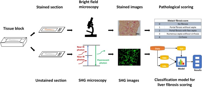
Figure 1
Schematic of study outline. Tissues were fixed, dehydrated, embedded in paraffin and sectioned into 2 consecutive slides. One was stained with Sirius Red (SR) for histological assessment by a patholog...
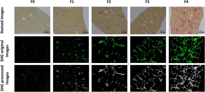
Figure 2
Representative images of SR-stained samples, SHG original images and SHG processed images at various stages of liver fibrosis.
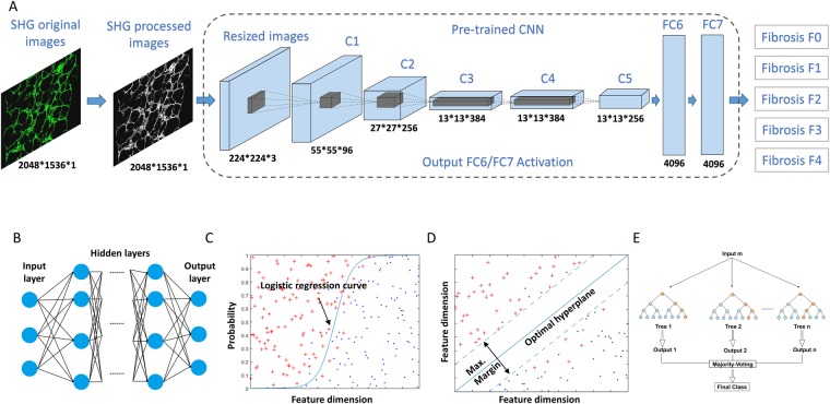
Figure 3
The architecture and of ( A ) deep learning via convolutional neuron networks (CNN) using pretrained 7-layered AlexNet and non-deep learning via ( B ) Artificial Neural Networks (ANN), ( C ) Multinomi...
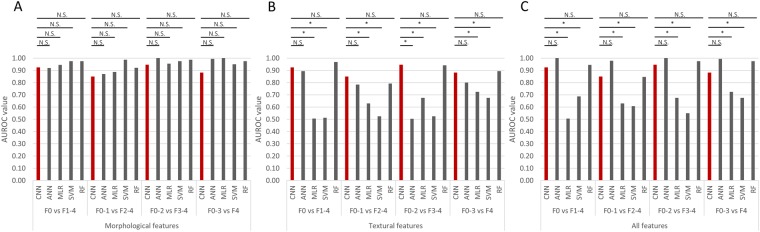
Figure 4
The area under receiver operating characteristic (AUROC) values for various classification models from AlexNet-Convolutional Neuron Networks (CNN), conventional Artificial Neural Networks (ANN), non-l...
Figure images are served from the NIH/NLM PubMed Central Open Access Subset or Europe PMC; copyright remains with the publishers and authors.
💬 Discussion
0 commentsNo comments yet. Be the first to start a discussion!
Leave a Comment