Abstract
AbstractHistological staining is a vital step in diagnosing various diseases and has been used for more than a century to provide contrast in tissue sections, rendering the tissue constituents visible for microscopic analysis by medical experts. However, this process is time consuming, labour intensive, expensive and destructive to the specimen. Recently, the ability to virtually stain unlabelled tissue sections, entirely avoiding the histochemical staining step, has been demonstrated using tissue-stain-specific deep neural networks. Here, we present a new deep-learning-based framework that generates virtually stained images using label-free tissue images, in which different stains are merged following a micro-structure map defined by the user. This approach uses a single deep neural network that receives two different sources of information as its input: (1) autofluorescence images of the label-free tissue sample and (2) a “digital staining matrix”, which represents the desired microscopic map of the different stains to be virtually generated in the same tissue section. This digital staining matrix is also used to virtually blend existing stains, digitally synthesizing new histological stains. We trained and blindly tested this virtual-staining network using unlabelled kidney tissue sections to generate micro-structured combinations of haematoxylin and eosin (H&E), Jones’ silver stain, and Masson’s trichrome stain. Using a single network, this approach multiplexes the virtual staining of label-free tissue images with multiple types of stains and paves the way for synthesizing new digital histological stains that can be created in the same tissue cross section, which is currently not feasible with standard histochemical staining methods.
🔬 Techniques
🔭 Microscopes
💻 Software
✨ Fluorophores
🧪 Sample Preparation
🏭 Microscope Brands
🔎 Objectives
💻 Software Details
💾 Data Repositories
🏛️ Research Organizations (ROR)
Affiliated research institutions:
📋 Methods
Data acquisition Unstained formalin-fixed and paraffin-embedded
(FFPE) kidney tissues were sectioned into thin, 2-μm slices and fixed on standard glass microscope slides. The training and validation dataset for each stain was made up of images obtained from 12-thin tissue sections acquired from unique patients. The test dataset was made up of four tissue sections from additional unique patients. Adjacent tissue sections from each of these patients were used for each of the three stains. Ethical approval for the use of these tissue sections was obtained under UCLA IRB number 18–001029. Using a conventional widefield fluorescence microscope (IX83, Olympus) equipped with a 20×/0.75 NA objective lens (Olympus UPLSAPO) and two separate filter cubes, DAPI (OSFI3-DAPI-5060C, EX 377/50 nm EM 447/60 nm, Semrock) and Texas Red (OSFI3-TXRED-4040C, EX 562/40 nm EM 624/40 nm, Semrock), autofluorescence imaging of these unlabelled tissue sections was performed. The tissue sections were neither deparaffinized nor cover-slipped before being imaged via fluorescence microscopy. The exposure time for the DAPI channel was 50 ms, and that for the Texas Red channel was 300 ms. Once the autofluorescence images had been obtained, the slides were histochemically stained using standard H&E, Jones’ silver or Masson’s trichrome stain and were then cover-slipped. The staining of the slides was performed by the UCLA Translational Pathology Core Laboratory (TPCL). The histochemically stained slides were then imaged using a scanning microscope (Aperio AT, Leica Biosystems, 20×/0.75NA objective with a 2× adapter) to create the target labels used to train, validate and test our neural network models. We used the two unlabelled autofluorescence images of the same tissue sample in conjunction with a digital staining matrix to select the stain or set of stains to be generated as the input to a neural network. This input was transformed by a class-conditional generative adversarial network into an equivalent image of a stained tissue section with the same field of view.
Show full methods section
Data acquisition Unstained formalin-fixed and paraffin-embedded
(FFPE) kidney tissues were sectioned into thin, 2-μm slices and fixed on standard glass microscope slides. The training and validation dataset for each stain was made up of images obtained from 12-thin tissue sections acquired from unique patients. The test dataset was made up of four tissue sections from additional unique patients. Adjacent tissue sections from each of these patients were used for each of the three stains. Ethical approval for the use of these tissue sections was obtained under UCLA IRB number 18–001029. Using a conventional widefield fluorescence microscope (IX83, Olympus) equipped with a 20×/0.75 NA objective lens (Olympus UPLSAPO) and two separate filter cubes, DAPI (OSFI3-DAPI-5060C, EX 377/50 nm EM 447/60 nm, Semrock) and Texas Red (OSFI3-TXRED-4040C, EX 562/40 nm EM 624/40 nm, Semrock), autofluorescence imaging of these unlabelled tissue sections was performed. The tissue sections were neither deparaffinized nor cover-slipped before being imaged via fluorescence microscopy. The exposure time for the DAPI channel was 50 ms, and that for the Texas Red channel was 300 ms. Once the autofluorescence images had been obtained, the slides were histochemically stained using standard H&E, Jones’ silver or Masson’s trichrome stain and were then cover-slipped. The staining of the slides was performed by the UCLA Translational Pathology Core Laboratory (TPCL). The histochemically stained slides were then imaged using a scanning microscope (Aperio AT, Leica Biosystems, 20×/0.75NA objective with a 2× adapter) to create the target labels used to train, validate and test our neural network models. We used the two unlabelled autofluorescence images of the same tissue sample in conjunction with a digital staining matrix to select the stain or set of stains to be generated as the input to a neural network. This input was transformed by a class-conditional generative adversarial network into an equivalent image of a stained tissue section with the same field of view.
Image pre-processing and co-registration
Because the purpose of the deep neural network was to learn the transformation from the unlabelled autofluorescence images of a tissue specimen to an image of a stained specimen, it was crucial that the FOVs were accurately aligned. Furthermore, since more than one autofluorescence channel was used as the network input, it was necessary to align the different filter channels. To use three different stains (H&E, Masson’s trichrome and Jones’s silver), we implemented image pre-processing and alignment for each pair of input and target images from the three staining datasets individually. The registration steps for matching the autofluorescence and bright-field images followed the process reported by Rivenson et al. 15 . One major addition is that when multiple autofluorescence channels (e.g., DAPI and Texas Red) are used as the network input, they must be aligned even if the images in both channels are captured using the same microscope; the corresponding FOVs from the two channels are not precisely aligned at the subpixel level, particularly at the edges of the FOVs. Therefore, we applied an elastic pyramidal registration algorithm to accurately align the multiple autofluorescence channels. This elastic registration algorithm matches the local features of two image channels by hierarchically breaking the image into increasingly smaller blocks and then matching the corresponding blocks 10 . The elastic registration algorithm begins by dividing the image into a grid of 5 × 5 blocks and calculating block-wise cross-correlations. The distance between the location with the peak correlation and the centre of the block is used to calculate the shift, as the area with the peak correlation is the point with maximum similarity between the two images. By using a weighted average of the translation vector for each block, a 2048 × 2048-pixel translation map was generated. This translation map was then applied to the Texas Red image to account for the differences between it and the DAPI image. To achieve accurate co-registration, the image was iteratively broken into increasingly smaller blocks until a block size of 100 × 100 pixels was reached. The final calculated transformation map was then applied to the Texas Red images to ensure that they were aligned with the corresponding images in the DAPI channel. An example of the use of this elastic transformation map can be seen in Fig. 5 . Finally, we stitched the aligned images from both channels to obtain whole-slide images of the samples that contained both the DAPI and Texas Red channels. Fig. 5 Example of co-registration between the DAPI and Texas Red image channels. The translation map was calculated using an elastic pyramidal registration algorithm and then applied to the Texas Red image channel. This process ensured that the two image channels were accurately co-registered with respect to each other Co-registration between the fluorescence and bright-field images began with global registration and proceeded with progressive alignment at smaller scales until subpixel-level co-registration was achieved. This first step of this process was to find a rough match by extracting the area of the bright-field image with the highest cross-correlation with a contrast-reversed version of the DAPI image. These images were then further aligned using MATLAB’s multimodal image registration feature 23 . Following this registration process, the neural network was trained using patches from these coarsely matched images. Using this network, the autofluorescence images were then virtually stained. However, because only coarse co-registration had been achieved at this point, the accuracy of the virtual staining results could not be satisfactory. Therefore, elastic pyramidal co-registration was then applied to match the histochemically stained images with the initial virtually stained images, resulting in a matched image pair. Before feeding the aligned pairs into the neural network, we implemented normalization on the whole-slide images generated from the DAPI and Texas Red images. This whole-slide normalization was performed by subtracting the mean value of the entire tissue sample and dividing by the standard deviation of the pixel values (note that background regions were excluded when calculating the mean and standard deviation). Deep neural network architecture, training and validation In this study, we used a class-conditional GAN architecture to learn the transformation from the label-free unstained autofluorescence input images to the corresponding bright-field image using three different stains (H&E, Masson’s trichrome and Jones’ silver). Following the co-registration of the autofluorescence images and the bright-field images, the accurately aligned FOVs were randomly partitioned into overlapping patches of 256 × 256 pixels and further augmented through rotation and flipping. The patches were then used to train the GAN. During the training process, this class-conditional GAN used a set of one-hot-encoded matrices, together referred to as the digital staining matrix, which was concatenated with the network’s 256 × 256 input image/image stack patches, with each matrix corresponding to a different stain. One way to represent this conditioning is: 2 documentclass[12pt]{minimal} usepackage{amsmath} usepackage{wasysym} usepackage{amsfonts} usepackage{amssymb} usepackage{amsbsy} usepackage{mathrsfs} usepackage{upgreek} setlength{oddsidemargin}{-69pt} begin{document}$$tilde c = left[ {c_1,c_2,c_3} right]$$end{document} c ~ = c 1 , c 2 , c 3 where [·] denotes concatenation and c i represents a 256 × 256 matrix of labels for the i -th stain type (in this example, H&E, Masson’s trichrome or Jones’ silver). For a pair of input and target images from the i -th stain dataset, c i was set to be an all-one matrix, while all remaining matrices were assigned values of zero. A GAN is composed of two deep neural networks, a generator and a discriminator (Fig. 6 ). During GAN training, the generator learns to perform a statistical transformation to generate a virtually stained image, while the discriminator attempts to distinguish between histochemically stained images and their virtually stained counterparts. The networks improve by learning from one another, improving the quality of the virtually stained images. For this task, we defined the loss functions of the generator and discriminator as: 3 documentclass[12pt]{minimal} usepackage{amsmath} usepackage{wasysym} usepackage{amsfonts} usepackage{amssymb} usepackage{amsbsy} usepackage{mathrsfs} usepackage{upgreek} setlength{oddsidemargin}{-69pt} begin{document}$$begin{array}{l}ell _{mathrm{generator}} = L_1left{ {{it{z}}_{mathrm{label}},Gleft( {x_{mathrm{input}},tilde c} right)} right} + lambda times {mathrm{TV}}left{ {Gleft( {{x}_{mathrm{input}},tilde c} right)} right} + alpha times left( {1 - D( {G( {x_{mathrm{input}},tilde c}),tilde c})} right)^2\ ell _{mathrm{discriminator}} = Dleft( {G( {x_{mathrm{input}},tilde c}),tilde c} right)^2 + left( {1 - D( {z_{mathrm{label}},tilde c})} right)^2end{array}$$end{document} ℓ generator = L 1 z label , G x input , c ~ + λ × TV G x input , c ~ + α × 1 − D ( G ( x input , c ~ ) , c ~ ) 2 ℓ discriminator = D G ( x input , c ~ ) , c ~ 2 + 1 − D ( z label , c ~ ) 2 where the total variation (TV) operator and mean absolute error ( L 1 -norm) are used to regularize the generator’s output and ensure that it is highly accurate. The TV operator and the L 1 -norm are defined as: 4 documentclass[12pt]{minimal} usepackage{amsmath} usepackage{wasysym} usepackage{amsfonts} usepackage{amssymb} usepackage{amsbsy} usepackage{mathrsfs} usepackage{upgreek} setlength{oddsidemargin}{-69pt} begin{document}$${mathrm{TV}}left( z right) = mathop {sum }limits_p mathop {sum }limits_q |z_{p, + ,1,q} - z_{p,q}| + |z_{p,q + 1} - z_{p,q}|$$end{document} TV z = ∑ p ∑ q ∣ z p + 1 , q − z p , q ∣ + ∣ z p , q + 1 − z p , q ∣ 5 documentclass[12pt]{minimal} usepackage{amsmath} usepackage{wasysym} usepackage{amsfonts} usepackage{amssymb} usepackage{amsbsy} usepackage{mathrsfs} usepackage{upgreek} setlength{oddsidemargin}{-69pt} begin{document}$$L_1left( {z,G} right) = frac{1}{{mathrm{P} times {mathrm{Q}}}}mathop {sum }limits_p mathop {sum }limits_q |z_{p,q} - Gleft( {x_{mathrm{input}},tilde c} right)_{p,q}|$$end{document} L 1 z , G = 1 P × Q ∑ p ∑ q ∣ z p , q − G x input , c ~ p , q ∣ where D (·) and G (·) refer to the outputs of the discriminator and generator networks, respectively; z label denotes the bright-field image of the histochemically stained tissue; and x input represents the input to the neural network. P and Q represent the numbers of vertical and horizontal pixels, respectively, of the image patch, and p and q represent the pixel locations. The regularization parameters ( λ and α ) were set to 0.02 and 2000, respectively, to accommodate a total variation loss term of approximately 2% of the L 1 loss and a discriminator loss term of 98% of the total generator loss. Fig. 6 Diagram showing the network architecture of the GAN used to perform the transformation. a Generator network. b Discriminator network For the generator a modified version of the U-net architecture was adopted 24 , as visualized in Fig. 6a . This U-net consists of four “down-blocks” followed by four “up-blocks”. Each of the down-blocks is made up of three convolutional layers and their activation functions, which together double the number of channels. These convolutional layers are followed by an average pooling layer with a stride and kernel size of two, which effectively down-samples the image. The up-blocks first bilinearly resize the tensors, up-sampling them by a factor of two. This is followed by three convolutional layers and their activation functions. These convolutional layers together reduce the number of channels by a factor of four. Between each of the up- and down-blocks of the same level, a skip connection is used. These skip connections concatenate the output of the down-blocks with the up-sampled values, allowing data to be passed at each level. Following these down- and up-blocks, a convolutional layer is used to reduce the number of channels to three, which correspond to the three colour channels in the bright-field image. The discriminator network, visualized in Fig. 6b , receives six input channels. Three channels (YCbCr colour map) come from either the generator output or the target/label, and three come from the one-hot-encoded digital staining matrix. The discriminator architecture contains a convolutional layer that transforms this input into a 64-channel feature map, which is, in turn, passed through a set of five blocks, each consisting of two convolutional layers and their corresponding activation functions. The second of these convolutional layers doubles the number of channels and has a stride of two. These five blocks are followed by two fully connected layers, which reduce the dimensionality to a single channel, which is acted upon by a sigmoid activation function. The convolutional filter size throughout the GAN is set to 3 × 3; the outputs of these filters are acted upon by the Leaky ReLU activation function, which is described as: 6 documentclass[12pt]{minimal} usepackage{amsmath} usepackage{wasysym} usepackage{amsfonts} usepackage{amssymb} usepackage{amsbsy} usepackage{mathrsfs} usepackage{upgreek} setlength{oddsidemargin}{-69pt} begin{document}$${mathrm{LeakyReLU}}left( x right) = left{ {begin{array}{*{20}{c}} !!!!!{x;mathrm{for};{it{x}}, > ,0} \ {0.1x;mathrm{otherwise}} end{array}} right.$$end{document} LeakyReLU x = x for x > 0 0.1 x otherwise During training, the learnable parameters were updated using the adaptive moment estimation (Adam) optimizer with learning rates of 1 × 10 −4 for the generator network and 2 × 10 −6 for the discriminator network. For each step of discriminator training, ten iterations of training were performed for the generator network. The batch size for training was set to 8. Virtual staining of unlabelled tissue images with a single stain Once the network had been trained, the one-hot-encoded label documentclass[12pt]{minimal} usepackage{amsmath} usepackage{wasysym} usepackage{amsfonts} usepackage{amssymb} usepackage{amsbsy} usepackage{mathrsfs} usepackage{upgreek} setlength{oddsidemargin}{-69pt} begin{document}$$tilde c$$end{document} c ~ was used to condition the network to generate the desired stained images. In other words, to generate solely the i -th stain, the matrix c i was set to be an all-one matrix, and the remaining matrices were set to be all zeros. Stain blending and micro-structured virtual staining of unlabelled tissue images Following the training process of the neural network model, we can use the conditional matrices in ways different to that in which the model was trained to virtually create new types of stains. The basic encoding rule that should be satisfied can be summarized as follows: 7 documentclass[12pt]{minimal} usepackage{amsmath} usepackage{wasysym} usepackage{amsfonts} usepackage{amssymb} usepackage{amsbsy} usepackage{mathrsfs} usepackage{upgreek} setlength{oddsidemargin}{-69pt} begin{document}$$mathop {sum }limits_{i = 1}^{N_{mathrm{stains}}} c_i,_j,_k = 1$$end{document} ∑ i = 1 N stains c i , j , k = 1 In other words, for a given set of indices j and k , the sum over the number of stains on which the network was trained ( N stains = 3 in our example) should be equal to 1. By modifying the class encoding matrices to use a mixture of multiple classes, the various stains can be blended, creating unique stains with features inherited from the various stains learned by the artificial neural network. Examples of such blended stains are illustrated in Fig. 4 . Another possible use of our trained multistain neural network is to partition the tissue field of view into different regions of interest (ROIs) and virtually stain each ROI using a different specific stain or blend of a sub-set of these stains: 8 documentclass[12pt]{minimal} usepackage{amsmath} usepackage{wasysym} usepackage{amsfonts} usepackage{amssymb} usepackage{amsbsy} usepackage{mathrsfs} usepackage{upgreek} setlength{oddsidemargin}{-69pt} begin{document}$$mathop {sum }limits_{i = 1}^{N_{mathrm{stains}}} c_i,_j,_k = 1, quadmathrm{for};{it{j,k}} subseteq mathrm{ROI}$$end{document} ∑ i = 1 N stains c i , j , k = 1 for j , k ⊆ ROI where ROI is the defined region of interest in the sample field of view. Multiple non-overlapping ROIs can be defined across a field of view, with different stains applied to different ROIs or micro-structures. These can be either defined by the user or algorithmically generated. As an example, a user can manually define various tissue areas via a graphical user interface and stain them with different stains. This will result in different tissue constituents being stained differently, as illustrated in Figs. 1 and 3 . We have implemented this ROI-selective staining (micro-structured staining) functionality using the Python segmentation package Labelme 25 . Using this package, we can generate logical masks in accordance with labelled ROIs, which are then processed to be the documentclass[12pt]{minimal} usepackage{amsmath} usepackage{wasysym} usepackage{amsfonts} usepackage{amssymb} usepackage{amsbsy} usepackage{mathrsfs} usepackage{upgreek} setlength{oddsidemargin}{-69pt} begin{document}$$tilde c_{ROI}$$end{document} c ~ R O I labels for specific microscopic areas. Other manual, software or hybrid approaches can also be used to implement the selection of certain tissue structures. Single-stain network used for SSIM calculations To generate virtually stained images using a single-stain network, a network with the same architecture but excluding the digital staining matrix was used. A separate network was trained for each of the three stains using the portion of the dataset specific to that stain. This single-stain network was implemented followed the approach previously reported 15 . Implementation details The virtual staining network was implemented using Python version 3.6.0, with the TensorFlow framework version 1.11.0. We implemented the software on a desktop computer with an Intel Xeon W-2195 CPU @2.30 GHz and 256 GB of RAM running the Microsoft Windows 10 operating system. Network training and testing were performed using a single NVIDIA GeForce RTX 2080 Ti GPU. The network was trained for 21,000 discriminator training steps over 47 h. Using a single GPU, inference can be performed at a rate of 3.9 s per 1 mm 2 of unlabelled tissue.
📊 Figures
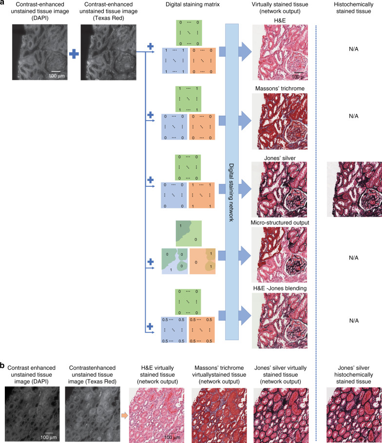
Fig. 1
Demonstration of multiple stains being virtually generated using a class-conditional neural network and images in two autofluorescence channels (DAPI and Texas Red) of a label-free tissue sample.
a Steps involved in virtually creating the various stains. By adding a class condition to the network using a digital staining matrix, a single network can be used to generate multiple stains or a ble...
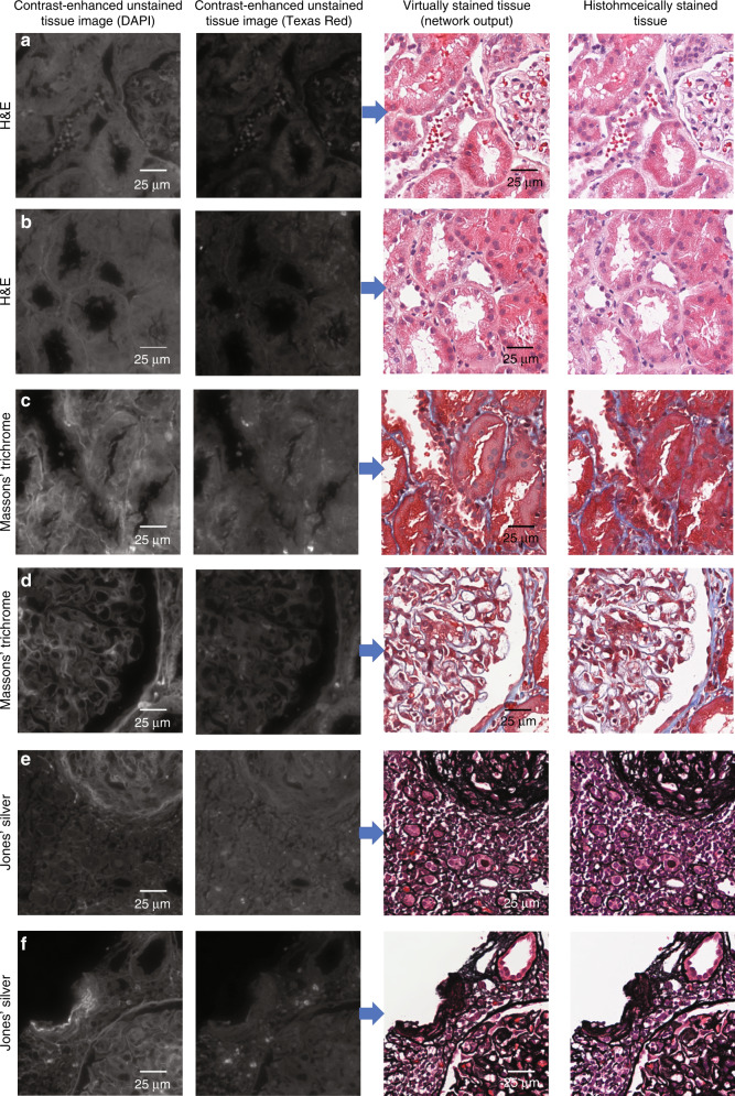
Fig. 2
Examples of various fields of view that have been virtually stained using the presented multistain network.
Co-registered histochemically stained fields of view of the same samples are also shown to the right, and the unstained autofluorescence images are shown to the left to permit direct comparison. a , b...
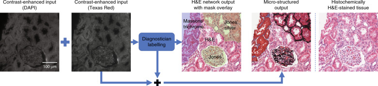
Fig. 3
Example of multistain micro-structuring.
Either a diagnostician or an algorithm can label sub-regions of the unstained tissue, creating on demand a digital staining matrix that defines the microscopic map of multiple stains to be virtually g...
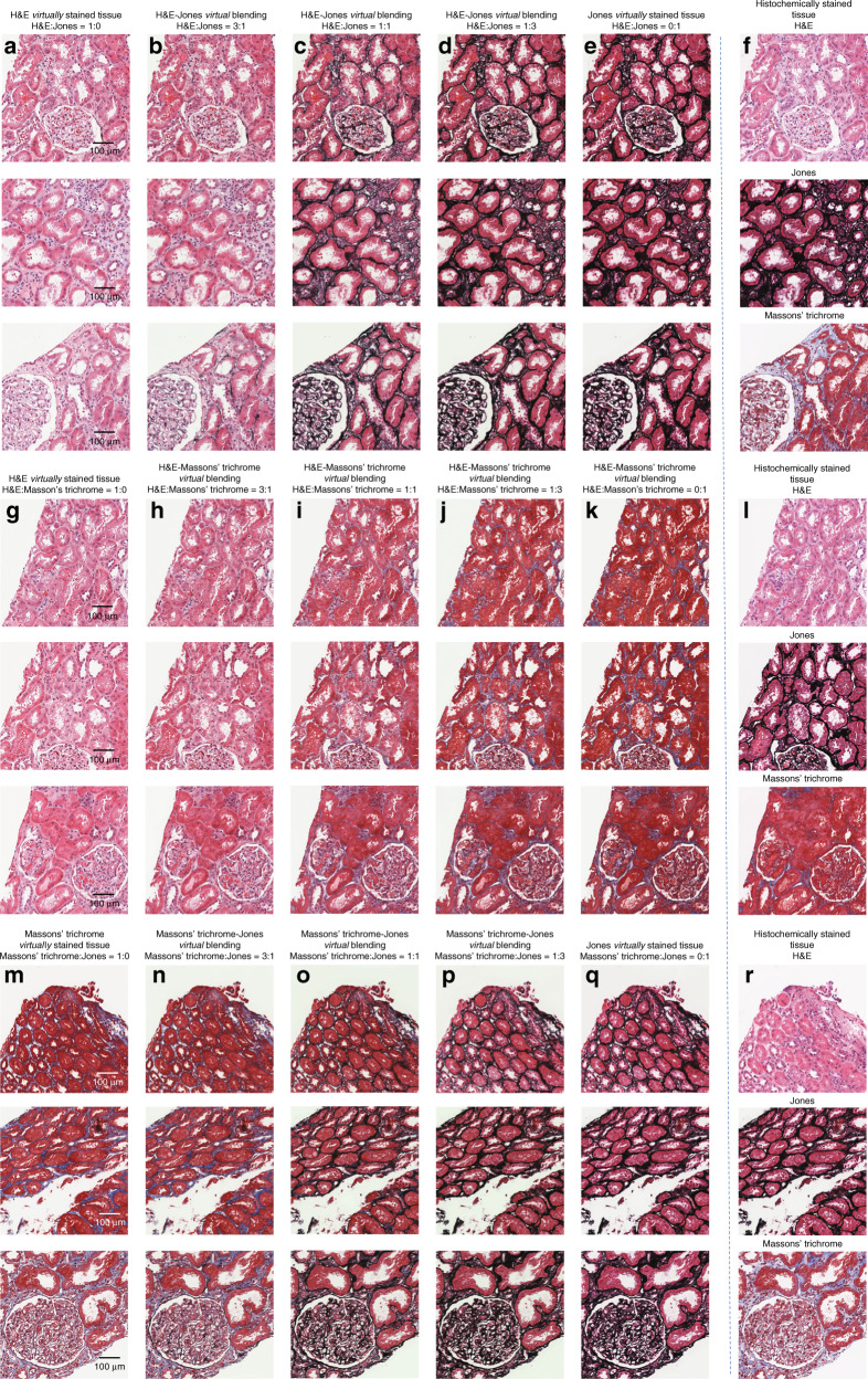
Fig. 4
Examples of stain blending.
a u2013 e Kidney tissue that has been virtually stained with varying class-condition ratios of H&E to Jonesu2019 silver stain. g u2013 k Kidney tissue that has been virtually stained with varying clas...
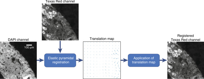
Fig. 5
Example of co-registration between the DAPI and Texas Red image channels.
The translation map was calculated using an elastic pyramidal registration algorithm and then applied to the Texas Red image channel. This process ensured that the two image channels were accurately c...
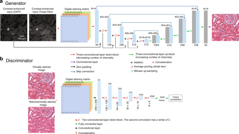
Fig. 6
Diagram showing the network architecture of the GAN used to perform the transformation.
a Generator network. b Discriminator network
Figure images are served from the NIH/NLM PubMed Central Open Access Subset or Europe PMC; copyright remains with the publishers and authors.
💬 Discussion
0 commentsNo comments yet. Be the first to start a discussion!
Leave a Comment