Abstract
The principles governing the functional organization and development of long-range network interactions in the neocortex remain poorly understood. Using in vivo widefield and two-photon calcium imaging of spontaneous activity patterns in mature ferret visual cortex, we find widespread modular correlation patterns that accurately predict the local structure of visually evoked orientation columns several millimeters away. Longitudinal imaging demonstrates that long-range spontaneous correlations are present early in cortical development before the elaboration of horizontal connections and predict mature network structure. Silencing feedforward drive through retinal or thalamic blockade does not eliminate early long-range correlated activity, suggesting a cortical origin. Circuit models containing only local, but heterogeneous, connections are sufficient to generate long-range correlated activity by confining activity patterns to a low-dimensional subspace via multisynaptic short-range interactions. These results suggest that local connections in early cortical circuits can generate structured long-range network correlations that guide the formation of visually evoked distributed functional networks.
🔬 Techniques
💻 Software
✨ Fluorophores
🧪 Sample Preparation
🏭 Microscope Brands
🧪 Reagent Suppliers
📷 Detectors
💻 Software Details
💾 Data Repositories
🏛️ Research Organizations (ROR)
Affiliated research institutions:
📋 Methods
Animals
All experimental procedures were approved by the Max Planck Florida Institute for Neuroscience Institutional Animal Care and Use Committee and were performed in accordance with guidelines from the US National Institutes of Health. 24 female ferret kits were obtained from Marshall Farms and housed with jills on a 16 h light/8 h dark cycle. See Supplementary table 1 for complete list of all animals used in each figure. No statistical methods were used to pre-determine sample sizes, but our sample sizes are similar to those reported in previous publications (e.g. refs 6 , 13 , 45 ).
Viral injections
Viral injections were performed as previously described 6 , 45 , 46 . Briefly we expressed GCaMP6s 47 by microinjecting AAV2/1.hSyn.GCaMP6s.WPRE.SV40 (obtained from University of Pennsylvania Vector Core) into visual cortex approximately 6–10 days prior to imaging experiments. Anesthesia was induced with either ketamine (12.5 mg/kg) or isoflurane (4–5%), and maintained with isoflurane (1–2%). Atropine (0.2mg/kg) and bupivacaine were both administered, and animal temperature was maintained at approximately 37°C with a homeothermic heating blanket. Animals were also mechanically ventilated and both heart rate and end-tidal CO2 were monitored throughout the surgery. Using aseptic surgical technique, skin and muscle overlying visual cortex were reflected and a small burr hole was made with a hand-held drill (Fordom Electric Co.). Approximately 1μL of virus contained in a pulled glass pipette was pressure injected into the cortex at two depths (~200 μm and 400 μm below the surface) over 20 minutes using a Nanoject-II (World Precision Instruments). This procedure reliably produced robust and widespread labelling of visual cortex, with GCaMP6 expression typically extending over an area >3 mm in diameter ( Supplementary Fig. 12 ).
Show full methods section
Animals
All experimental procedures were approved by the Max Planck Florida Institute for Neuroscience Institutional Animal Care and Use Committee and were performed in accordance with guidelines from the US National Institutes of Health. 24 female ferret kits were obtained from Marshall Farms and housed with jills on a 16 h light/8 h dark cycle. See Supplementary table 1 for complete list of all animals used in each figure. No statistical methods were used to pre-determine sample sizes, but our sample sizes are similar to those reported in previous publications (e.g. refs 6 , 13 , 45 ).
Viral injections
Viral injections were performed as previously described 6 , 45 , 46 . Briefly we expressed GCaMP6s 47 by microinjecting AAV2/1.hSyn.GCaMP6s.WPRE.SV40 (obtained from University of Pennsylvania Vector Core) into visual cortex approximately 6–10 days prior to imaging experiments. Anesthesia was induced with either ketamine (12.5 mg/kg) or isoflurane (4–5%), and maintained with isoflurane (1–2%). Atropine (0.2mg/kg) and bupivacaine were both administered, and animal temperature was maintained at approximately 37°C with a homeothermic heating blanket. Animals were also mechanically ventilated and both heart rate and end-tidal CO2 were monitored throughout the surgery. Using aseptic surgical technique, skin and muscle overlying visual cortex were reflected and a small burr hole was made with a hand-held drill (Fordom Electric Co.). Approximately 1μL of virus contained in a pulled glass pipette was pressure injected into the cortex at two depths (~200 μm and 400 μm below the surface) over 20 minutes using a Nanoject-II (World Precision Instruments). This procedure reliably produced robust and widespread labelling of visual cortex, with GCaMP6 expression typically extending over an area >3 mm in diameter ( Supplementary Fig. 12 ).
Cranial window surgery
To allow repeated access to the same imaging field, chronic cranial windows were implanted in each animal 0–2 days prior to the first imaging session. Animals were anesthetized and prepared for surgery as described above. Using aseptic surgical technique, skin and muscle overlying visual cortex were reflected and a custom-designed metal headplate was implanted over the injected region with MetaBond (Parkell Inc.). Then both a craniotomy (~5mm) and a subsequent durotomy were performed, and the underlying brain stabilized with a 1.4 mm thick 3 mm diameter stacked glass coverslip 46 . The headplate was hermetically sealed with a stainless steel retaining ring (5/16” internal retaining ring, McMaster-Carr) and glue (VetBond, 3M). Unless the animal was immediately imaged after a cranial window surgery, the imaging headplate was filled with a silicone polymer (Kwik-kast, World Precision Instruments) to protect it between imaging experiments.
Wide-field epifluorescence and two-photon imaging
Wide-field epifluoresence imaging was achieved with a Zyla 5.5 sCMOS camera (Andor) controlled by μManager 48 . Images were acquired at 15Hz with 4 × 4 binning to yield 640 × 540 pixels. Two-photon imaging was performed with a B-Scope microscope (ThorLabs) driven by a Mai-Tai DeepSee laser (Spectra Physics) at 910 nm. The B-Scope microscope was controlled by ScanImage (Vidreo Technologies) in a resonant-galvo configuration with single-plane images (512 × 512 pixels) being collected at 30 Hz. In animals imaged after eye opening, phenylephrine (1.25–5%) and tropicamide (0.5%) were applied to the eyes to retract the nictitating membrane and dilate the pupil, and the cornea was protected with regular application of eye drops (Systane Ultra, Alcon Laboratories). The silicon polymer plug overlying the sealed imaging chamber was then gently peeled off. Whenever the imaging quality of the chronic cranial window was found to be suboptimal for imaging, the chamber was opened under aseptic conditions, regrown tissue or neomembrane was removed and a new coverslip was inserted. In some cases, prior to imaging, animals were paralyzed with either vecuronium or pancuronium bromide (0.2 mg/kg/h in lactated Ringer’s, delivered IV). For imaging experiments in awake animals, animals were habituated to head fixation beginning at least 2 days before imaging. Habituation consisted of exposure to the fixation apparatus for brief periods after which animals were returned to their home cage. For imaging, animals were head fixed and wide-field and two-photon imaging was performed as above. In experiments where both awake and anesthetized imaging were performed, awake imaging was always performed first, followed by anesthesia induction as described above. Awake recordings of spontaneous activity were performed in a darkened room and eye position not monitored. For anesthetized, longitudinal imaging experiments, anesthesia was induced with either ketamine (12.5 mg/kg) or isoflurane (4–5%), and atropine (0.2mg/kg) was administered. Animals were intubated and ventilated, and an IV catheter was placed in the cephalic vein. In some imaging sessions, it was not possible to catheterize the cephalic vein; in these cases, an IP catheter was inserted. Anesthesia was then maintained with isoflurane (0.5–0.75%). Following imaging, animals were recovered from anesthesia and returned to their home cages. During recovery, neostigmine was occasionally administered to animals that were paralyzed (0.01–0.1μL/kg per dose).
Visual stimulation
Visual stimuli were delivered on a LCD screen placed approximately 25–30cm in front of the eyes using PsychoPy 49 . For evoking orientation responses, stimuli were full-field sinusoidal gratings at 100% contrast, at 0.015–0.06 cycles per degree, drifting at 1 or 4 Hz, and presented at each of eight directions of motion, for 5s, repeated 8–16 times. In addition, “blank” stimuli of 0% contrast were also presented. Stimuli were randomly interleaved and were presented for 5s followed by a 5–10s gray screen. Spontaneous activity was recorded in a darkened room, with the visual stimulus set to a black screen.
Analysis software
Data analysis was performed in Python, ImageJ, and Matlab (The Mathworks).
Signal extraction for wide-field epifluorescence imaging
To correct for mild brain movement during imaging (especially in the awake state), we registered each imaging frame by maximizing phase correlation to a common reference frame. Furthermore, all imaging experiments acquired during a single day were registered into one reference frame. The ROI was manually drawn around the cortical region with high and robust visually evoked activity. The baseline F0 for each pixel was obtained by applying a rank-order filter to the raw fluorescence trace with the rank between 15 to 70 and the time window between 10 and 30s (values chosen for each imaging session individually, depending on the strength of spontaneous activity). The rank and time window were chosen such that the baseline followed faithfully the slow trend of the fluorescence activity. The baseline corrected spontaneous activity was calculated as (F-F0)/F0 = ΔF/F0. The baseline for each pixel for the visually evoked activity was obtained by taking the averaged last 1s of the inter-stimulus interval immediately before stimulus onset. The grating evoked response was then calculated as being the average of the fluorescence ΔF/F0 over the full stimulus period (5s).
Event detection
To detect spontaneously active events, we first determined active pixels on each frame using a pixel-wise threshold set to 4–5 standard deviations above each pixel’s mean value across time. Active pixels not part of a contiguous active region of at least 0.01mm 2 were considered ‘inactive’ for the purpose of event detection. Active frames were taken as frames with a spatially extended pattern of activity (>80% of pixels were active). Consecutive active frames were combined into a single event starting with the first high activity frame and then either ending with the last high activity frame or, if present, an activity frame defining a local minimum in the fluorescence activity. In order to assess the spatial pattern of an event, we extracted the maximally active frame for each event, defined as the frame with the highest activity averaged across the ROI. Importantly, calculating the spontaneous correlation patterns (see below) over all frames of all events preserves their spatial structure ( Supplementary Fig. 13 ). Imaging sessions in which less than 10 spontaneous events were detected were excluded from further analysis. This threshold was chosen based on randomly sampling (with replacement) a varied number of activity patterns, which revealed that spontaneous correlation patterns (see below) for subsamples of >10 events were highly similar (second-order correlation >=0.5) to those obtained from all events ( Supplementary Fig. 14 ). Spontaneous correlation patterns To assess the spatial correlation structure of spontaneous activity, we applied a Gaussian spatial high-pass filter (with SD of Gaussian filter kernel s high =195μm) to the maximally active frame in each event and down-sampled it to 160 × 135 pixels. The resulting patterns, named spontaneous patterns A in the following, were used to compute the spontaneous correlation patterns as the pairwise Pearson’s correlation between all locations x within the ROI and the seed point s 1 C ( s , x ) = 1 N ∑ i = 1 N ( A i ( s ) − A ( s ) ) ( A i ( x ) − 〈 A ( x ) 〉 ) σ s σ x Here the brackets < > denote the average over all events and σ x denotes the standard deviation of A over all N events i at location x . Note that the spatial structure of spontaneous activity was already evident without filtering ( Supplementary Fig. 15 ). High-pass filtering allowed us to extract this spatial structure, but our results did not sensitively depend on the filtering. For instance, weaker high-pass filtering using a kernel with s high =520μm resulted in a highly similar correlation structure (data not shown). Shuffled control ensemble and surrogate correlation patterns We compared the real ensemble of spontaneous activity patterns from a given experiment with a control ensemble, obtained by eliminating most of the spatial relationship between the patterns. To this end, all activity patterns were randomly rotated (rotation angle drawn from a uniform distribution between 0° and 360° with a step size of 10°), translated (shifts drawn from a uniform distribution between ±450 μm in increments of 26 μm, independently for x- and y-direction) and reflected (with probability 0.5, independently at the x- and y-axis at the center of the ROI), resulting in an equally large control ensemble with similar statistical properties, but little systematic interrelation between patterns. Surrogate correlation patterns were then computed from these ensembles as described above. Spatial range of correlations To assess the spatial range of spontaneous correlations ( Figs. 1e and 3d ), we identified the local maxima (minimum separation between maxima 800 μm) in the correlation pattern for each seed point and fitted an exponential decay function 2 f ( x ) = e − x ξ ( 1 − c 0 ) + c 0 to the values of these maxima as a function of distance x to the seed point ( Fig. 1e ; Supplementary Fig 9a ). Here ξ is the decay constant, named ‘spatial scale correlation’ in Fig. 4d and 7c-f . The baseline c 0 accounts for spurious correlations due to a finite number of spontaneous patterns and was estimated as the average value at maxima in the surrogate correlation patterns described above. To assess the statistical significance of long-range correlations ~2 mm from the seed point, we compared the median correlation strength for maxima located 1.8–2.2 mm away against a distribution obtained from 100 surrogate correlation patterns. For individual animals, the p-value was taken as the fraction of median correlation strength values from surrogate data greater than or equal to the median correlation strength for real correlation patterns. For 2 of 12 animals, the statistical significance of long-range correlations could not be assessed, due to insufficient coverage in rotated and translated surrogate activity patterns caused by an irregularly shaped ROI. These animals were excluded from analysis of long-range correlation strength. Comparison of awake and anesthetized correlations Correlation similarity across awake and anesthetized states was computed for each seed-point as the Pearson’s correlation coefficient of the spontaneous correlations for that seed point across states. For each seed-point, correlations within 400 μm were excluded from analysis. These “second-order correlations” (shown for each seed point in Supplementary Fig. 4f ) were then averaged across all seed points within the ROI. To determine the significance of these second-order correlations across state, we shuffled corresponding seed points across states 1000 times, and again computed correlation similarity. Likewise, to gain an estimate of the expected similarity for a well-matched correlation structure, we computed the similarity of each state to itself. Correlation patterns were first separately computed for half of the detected events, and then the two patterns were compared as above. Comparison of wide-field and cellular correlations 2-photon images were corrected for in plane motion via a 2D cross correlation-based approach. For awake imaging, periods of excessive motion were discarded and excluded from further analysis. Cellular regions of interest (ROIs) were drawn using custom software (Cell Magic Wand, 50 ) in ImageJ and imported into Matlab via MIJ 51 . Fluorescence was averaged over all pixels in the ROI and traces were converted to ΔF/F0 6 , where the baseline fluorescence, F0, was computed from a filtered fluorescence trace. The raw fluorescence trace was filtered by applying a 60 s median filter, followed by a first-order Butterworth high-pass filter with a cut-off time of 60 s. To compute spontaneous correlations ( Fig. 1f, g ), we first identified frames containing spontaneous events, which were defined as frames in which > 30% of imaged neurons exhibited activity > 2 standard deviations above their mean. The stability of activity during an event was computed as the cross-correlation of each frame with the peak activity frame, and was compared to a distribution of 100 randomly chosen intervals of the same length. Cellular activity on all event frames was then Z-scored using the mean and standard deviation of each frame, and correlation patterns for each cell were computed as the pairwise Pearson’s correlation coefficient, using the activity of all neurons on all active frames. To compare the correlation structure obtained at the cellular level with that obtained via wide-field imaging ( Fig. 1g ) we first aligned the 2-photon field of view (FOV) to the wide-field image using blood vessel landmarks and applied an affine transformation to obtain the pixel coordinates of each imaged neuron in the wide-field frame of reference. Correlation similarity was obtained as above by computing the second-order correlation between the cellular correlation structure and that of the corresponding wide-field pixels, using all cells >200μm from the seed point. Shuffled second-order correlations were obtained by randomly rotating and translating the 2P FOV within the full wide-field ROI, 1000 times. To estimate the maximum expected degree of similarity, we computed a second-order correlation within the cellular correlation structure itself by determining the similarity of correlation structures computed using only 50% of detected events (dashed line and blue bar in Fig. 1i ). Orientation preference and ocular dominance maps The orientation preference maps ( Fig. 2a , 5a ( right )) were calculated based on the trial-averaged responses evoked by binocularly presented moving grating stimuli of eight directions equally spaced between 0 and 360 degree. Responses were Gaussian band-pass filtered (SD: s low =26μm, s high =195μm) and orientation preference was computed by vector summation: 3 z ( x ) = ∑ k = 1 8 w k ( x ) e 2 i ϕ k w i t h x = ( x , y ) T where w k ( x ) is the tuning curve at location x , i.e. the trial-averaged response to a moving grating with direction ϕ k at location x . The preferred orientation at x is 0.5 arg (z( x )) . Orientation pinwheel centers ( Fig 2i, j ) were estimated as described in Refs. 52 , 53 . The Matlab routine provided by Schottdorf et al. (Ref. 53 ). was used. Orientation contour lines ( Fig. 2b , 5a ) are the zero-levels of the 0°−90° difference map, obtained by using the matplotlib.pyplot.contours routine. Surrogate orientation preference maps were obtained by phase shuffling the original maps in the Fourier domain 52 . Ocular dominance maps were calculated based on the trial-averaged responses evoked by presenting moving grating stimuli of eight directions equally spaced between 0 and 360 degree either to the contralateral or ipsilateral eye. The trial averaged response to each orientation and ocular condition was Gaussian band-pass filtered as described above for the orientation map. Contralateral and ipsilateral response maps were computed by respectively averaging together the trial-average responses to the stimuli presented either to the contralateral or ipsilateral eye. The ocular dominance map was computed as a difference of the contralateral and ipsilateral response maps. Similarity of correlation patterns to the orientation and ocular dominance maps To quantify how similar patterns of correlated spontaneous activity are to known functional maps in visual cortex, we computed the average pairwise similarity of the spontaneous correlation patterns either to the ocular dominance map or the orientation preference map ( Supplementary Fig. 5 ). The assessment of similarity of each correlation pattern to the ocular dominance map is the magnitude of their pairwise coefficient: 4 r O D ( x ) = | c o r r ( O D ( y ) , C ( x , y ) ) | where OD( y ) is the ocular dominance map at location y and C( x, y ) is the spontaneous correlation pattern between seed location x and location y and corr denotes Pearson’s correlation coefficient. Correspondingly, the similarity of each correlation pattern to the orientation map is computed as the magnitude of the pairwise correlation coefficient to the real and imaginary components of the vector-summed orientation map z : 5 r OP ( x ) = c o r r ( Re ( z ( y ) ) , C ( x , y ) ) 2 + c o r r ( Im ( z ( y ) ) , C ( x , y ) ) 2 Prediction analysis and exclusion areas To test whether orientation tuning can be predicted from the tuning at remote locations with correlated spontaneous activity ( Fig. 2c ), we estimated the tuning curve at seed point s =(s x , s y ) by the sum over tuning curves w k at different locations weighted by their spontaneous correlation C with the seed point: 6 w k p r e d ( s ) = ∑ x w k ( x ) C ( s , x ) where k denotes the orientation of the stimulus. The sum was taken over locations x outside a circular area centered at the seed point with radius 0.4, 1.2 or 2.4mm. For this calculation, both w k and C are z-scored. To assess the goodness of the prediction, we calculated the angular difference between the predicted and the actual preferred orientation ( Fig. 2f ). Low values indicate a high match, whereas 45° indicates chance level. Statistical significance ( Fig. 2f ) was determined by repeating this analysis for 100 surrogate orientation preference maps, obtained by phase shuffling in the Fourier domain 52 . For individual animals, the p-value was taken as the fraction of values equal or smaller than the value for the real orientation map. To pool across animals within an exclusion radius ( Fig. 2f ), we then generated 10,000 surrogate group medians by randomly drawing from the distributions of surrogate data points (one per animal), and the p-value was taken as the fraction of group medians equal or smaller than the median value for the actual data. Spontaneous fractures Fracture strength was defined as the rate by which the correlation pattern changes when changing the seed point location over some small distance ( Fig. 3b ( bottom ), Fig. 3c ). It was computed as: 7 F ( s ) = F d x ( s ) 2 + F dy ( s ) 2 where F dx ( F dy ) denotes the x(y)-component of the rate of change of the correlation pattern at seed point s . We approximated this rate of change by the (second-order) correlation between two correlation patterns with seed points at adjacent pixels a distance d apart: 8 F dy ( s ) = 1 − C dy ( s ) d 9 C dy ( s ) = c o r r x ( C ( s , x ) , C ( s + d e y , x ) ) where corr x denotes Pearson’s correlation coefficient calculated over all locations x and e y is a unit vector in y-direction. The subtraction from 1 in the numerator ensures F=0 at seed point locations, around which the correlation pattern does not change, while high values of F indicate high changes. We used d =26 μm, the spatial resolution of the correlation patterns. We defined fracture magnitude ( Supplementary Fig. 9c,d , Supplementary Fig. 10f ( bottom ), Supplementary Fig. 11b ) as the difference between F , averaged over the fracture lines, and its average in regions > 130μm apart from the nearest fracture line. To extract the fracture lines from F we first applied a spatial median filter with a window size of 78μm to remove outliers. We then applied histogram normalization, contrast enhancement by using Contrast Limited Adaptive Histogram Equalization (CLAHE, clip limit=20, size of neighborhood 260×260 μm 2 ), and a spatial high-pass filter (Gaussian filter, SD s high =390 μm). The resulting values were binarized (threshold=0), and the resulting two-dimensional binary array eroded and then dilated (twice) to remove single not-contiguous pixels. We skeletonized this binary array to obtain the fracture lines. We quantified the co-alignment between spontaneous fractures and high orientation gradient regions by the fracture selectivity ( Fig. 3e ), defined as the difference between F at high orientation gradient locations ( x high , >π/5 radians/pixel) and locations far from high orientation gradients ( x low , >150μm from x high ): 10 F S = 〈 F ( x h i g h ) 〉 − 〈 F ( x l o w ) 〉 〈 F ( x h i g h ) 〉 + 〈 F ( x l o w ) 〉 where the brackets denote average over locations x high and low x low , respectively. A value of FS of 1 indicates co-alignment between the spontaneous fractures and the orientation gradient, whereas a value near 0 indicates no such alignment. To assess significance ( Fig. 3e ) we repeated this analysis for 1000 surrogate orientation preference maps, obtained by phase shuffling in the Fourier domain. The p-value is the fraction of values equal or larger than the value for the orientation map. In order to test whether spontaneous fractures reflect the correlation structure over remote distances and not only in their local neighborhood ( Fig. 3c ( top ), Fig. 3f ), we computed F as above, but excluding a circular region with radius 0.4, 1.2 or 2.4 mm, centered at the seed point s . We then computed the Pearson’s correlation coefficient with the original F .
Registration for longitudinal imaging
To compare spontaneous correlation patterns across days in longitudinally imaged animals, we transformed all imaging data into a common reference frame ( Supplementary Fig. 6a ). This transformation corrected for small displacement and expansion of cortical tissue over the imaging period, presumably due to cortical growth. We used an affine transformation, thereby taking into account rotation, scaling, translation and shear mapping of the cortex: 11 x ' = T x + h 12 w i t h T = ( a b c d ) , 13 h = ( e , f ) T The parameter of the transformation matrix T and of the displacement vector h were found by minimizing the distance between landmarks determined for each day of experiment. Landmarks were found by marking radial blood vessels (i.e. blood vessels oriented orthogonally to the imaging plane) by visual inspection. The following expression was minimized (least square fit) to find transformation parameters from day t to the reference day t ref (eye opening): 14 ∑ i = 1 N ( X t r e f ,i − x t , i i ) 2 = ∑ i = 1 N ( x t r e f , i − Tx t , i − h ) 2 with N landmarks (between 10 to 30) in both coordinate systems at coordinates x tref,i in the reference coordinate system, and the coordinates x t,i at day t .
Analysis of spontaneous correlation across development
To compare spontaneous correlation patterns across development, we calculated a second-order correlation ( Supplementary Fig. 6d,e ) between the correlation patterns on a given day and the reference day (eye opening) with the same seed point. Changes in correlation fractures over development were quantified as the second order correlation of fracture patterns ( Supplementary Fig. 6f ). In both cases, an estimate of the expected degree of similarity was computed by first separately computing correlations and their corresponding fracture patterns for half of the detected events, and then computing the second-order correlations as above. To determine whether correlation patterns early in development can predict mature orientation preferences ( Fig. 5c ), we computed orientation tuning predictions as above, using the correlation pattern on a given day to weight tuning curves measured following eye opening, with an exclusion radius of 400 μm. The predicted orientation preference map was compared to the actual map as described above (“Prediction analysis and exclusion areas”) for both individual animals and group medians. To assess the statistical significance of long-range correlation strength at 2 mm across development, we compared correlation maxima to those of surrogate correlation patterns as described above (“Spatial range of correlations”). To pool across experiments within an age group, we then generated 10,000 surrogate group medians by randomly drawing from the distributions of surrogate data points (one per experiment), and the p-value was taken as the fraction of group medians greater than the median value for the actual data. Retinal and LGN inactivation experiments For retinal inactivation experiments, a cranial window was implanted over visual cortex as described above. After imaging spontaneous activity under light isoflurane anesthesia (0.5–1%) as described above, visually evoked responses were recorded in response to full-field luminance steps 6 . Isoflurane levels were then increased and intraocular infusions of TTX were performed into each eye. For each intraocular injection, a small incision was made just posterior to the scleral margin using the tip of a 30-gauge needle attached to a Hamilton syringe. Each eye was then injected with 2–2.5 μL of 0.75 mM TTX solution (Tocris Bioscience) to reach an intraocular dose of 21.45 μM that is roughly comparable the dosage used previously in the ferret 54 . Following infusion of TTX, isoflurane levels were reduced, and the animal returned to a stable light anesthetic plane. The efficacy of TTX was tested by the absence of visually evoked responses to full-field luminance steps. Following confirmation of retinal blockade, spontaneous activity was imaged as above. Following collection of spontaneous activity, retinal blockade was again confirmed through the absence of cortical responses to visual stimuli. For LGN inactivation experiments, surgical preparation was as described above. A head-post was implanted near bregma, a craniotomy was made over visual cortex, and sealed with a coverslip affixed directly to the skull with cyanoacrylate glue and dental cement. A second craniotomy was then made over the approximate location of the LGN (Horsley-Clarke coordinates: AP −1mm, LM 6mm). The LGN was typically located at a depth of 5–8.5mm, and its spatial position mapped by identifying units responsive to a full-field luminance stimulus through systematic electrode penetrations. Once the LGN position was determined, spontaneous activity in visual cortex was recorded as above, followed by visually-evoked responses to luminance steps. A micropipette filled with muscimol (25–100 mM, Tocris Biosciences) was lowered into the center of the LGN, and infusions of ~0.5 μL were made at three depths along the dorsal-ventral extent of the penetration using a nanoliter injector (Nanoject). The efficacy of thalamic inactivation was confirmed by the abolishment of visually evoked activity prior to and following imaging of spontaneous activity in the cortex. Spontaneous activity was analyzed as described above, with one exception: the 10 event threshold for inclusion (see above) was not applied to the LGN inactivation experiments as in 1 of 3 cases and standard deviation σ ε both depending linearly on H (< ε>=H, σ ε = 0.13 H ). The size of σ 1 was drawn from a normal distribution with SD 0.1< σ 1 > H and mean < σ 1 >=1.8. The orientation φ of the Mexican hat axis was drawn from a uniform distribution between 0° and 180°. These three parameters were drawn independently at each location. In the case of isotropic Mexican hat connectivity ( σ 1 = σ 2 ) the eigenvectors of M are plane waves and the spectrum is peaked at the wavenumber k =2π/ Λ , and thus the typical spatial scale Λ of the pattern is given by 20 Λ 2 = 4 π 2 σ 1 2 ( κ 2 − 1 ) 4 In ( κ ) This defines the spatial scale Λ used as reference in Fig. 7b,c . For comparison between model and data we identified 1 Λ with 1mm, which is roughly the spatial scale of spontaneous patterns observed in experiment. The input drive I is assumed constant in time for simplicity, consistent with our observation that in the early cortex spontaneous patterns were often fairly static during a spontaneous event ( Supplementary Figure 2 and Video 5 ). I is modulated in space using a band-pass filtered Gaussian random field G with spatial scale Λ, zero mean and unit SD 52 : 21 I ( x ) = 1 + η G ( x ) We varied the input modulation η between 0.004 and 0.4 in Figs. 4k,l the regime over which we observed a smooth transition from an input-dominated system to a system dominated by the recurrent connections. To model a spontaneous event, we integrated eq. 18 until a near steady state of the dynamics was reached. The results in Fig. 7c-h were obtained for an integration time of 500 τ , but already a much shorter integration over 50 τ resulted in similar solutions and nearly the same level of long-range correlations and dimensionality. Different spontaneous events were obtained by using different realizations of input drive I and initial conditions (same connectivity M ). To generate Figs. 7d,g,h and Supplementary Figs. 9b,d,f,h and 11 we furthermore averaged over 10 realizations of connectivity M for each parameter setting. We numerically integrated the dynamics using a 4 th order Runge-Kutta method in a square region of size 100 × 100 using periodic boundary conditions. The time step was dt =0.15 τ and the spatial resolution 10 pixel per Λ . The simulations were performed on the GPUs GeForce GTX TITAN Black and GeForce GTX TITAN X. The code was implemented in Python and Theano (version 0.8.1). Model of excitatory and inhibitory neural population To investigate whether modular activity and long-range correlations can be generated without Mexican hat connectivity, we generated an excitatory / inhibitory two-population model. Building on previous work 39 , 40 , the model consists of an excitatory and an inhibitory neural population and neurons are linked via local lateral connections (with Gaussian profiles). We consider a regime, in which the range of connections formed by excitatory neurons is more than 30% larger than that of inhibitory neurons. Spontaneous activity in the early visual cortex is modelled by the following dynamics: 22 τ du e ( x , t ) d t = − u e ( x , t ) + [ γ ∑ y ( M ee ( x , y ) u e ( y , t ) − M ei ( x , y ) u i ( y , t ) ) + J e ( x ) ] + , 23 τ d u i ( x , t ) d t = − u i ( x , t ) + [ γ ∑ y ( M ie ( x , y ) u e ( y , t ) − M ii ( x , y ) u i ( y , t ) ) + J i ( x ) ] + , 24 [ x ] + = { x i f x ≥ 0 0 o t h e r w i s e where u e (x,t) ( u i (x,t) ) is the average firing rate of an excitatory (inhibitory) unit at location x in a two-dimensional model cortex. τ is the neuronal time constant and assumed to be the same for excitatory and inhibitory units. M mn ( x,y ) are the synaptic weights connecting location y in population n to location x in population m ( m,n є { e,i }, with e being the excitatory and i the inhibitory population). The sum goes over all locations y within the network. γ is a factor controlling the overall strength of synaptic weights. Both excitatory and inhibitory units cover space uniformly and with equal density. J m ( x ) is the input to location x in population m . The connectivity matrix M consists of the four synaptic weight matrices M mn ( x , y ) that are assumed to be short-range and modelled by isotropic Gaussians: 25 M ( x , y ) = ( M ee ( x , y ) − M ei ( x , y ) M ie ( x , y ) − M i i ( x , y ) ) 26 M mn ( x , y ) = M mn ( | x − y | ) = a mn 2 πσ mn 2 exp ( − | x − y | 2 2 σ mn 2 ) , m , n ϵ { e , i } Here σ mn denotes the SD and a mn the strength of the Gaussian that connects population n to m . The a mn were normalized such that the maximal eigenvalue of M is equal to 1. Note that the Gaussian connectivity profile is isotropic and identical for all units. Thus, the network connectivity exhibits rotation and translation symmetry. To model a spontaneous event, we assumed an input drive constant in time and space with a value J e ( x ) = J i ( x ) = J = 1. We set τ =1, γ =1.02 and used random initial conditions u e ( x ,t=0) , u i ( x ,t=0) drawn from a Gaussian distribution with zero mean and unit SD rectified at zero. The parameters for the connectivity were set to a ee = 22.2 , a ie =a ei = 21.6 , a ii = 20.8 , σ ee =σ ie = 1.9 , σ ei = 1.4 , σ ii = 0.6. (Changing these values by 10% produced qualitatively similar results.) We integrated the network dynamics until a near steady state of the dynamics was reached. The results in Supplemental Figs. 8d-h , 11 were obtained for an integration time of 500 τ . Different spontaneous events were obtained by using different initial conditions (same connectivity M and input J ). We numerically integrated the dynamics using a 4th order Runge-Kutta method in a square region of size 80 × 80 using periodic boundary conditions and a time step dt=0.15 τ . As above, the simulations were performed on the GPUs GeForce GTX TITAN Black and GeForce GTX TITAN X. The code was implemented in Python and Theano (version 0.8.1). In our numerical simulations, hexagonal activity patterns occurred for a broad range of connectivity parameters. For specific choices of parameter combinations, we could even obtain this type of solution when setting σ ii to a similar value as σ ei , so that the range of connectivity from inhibition to excitation is similar to that from inhibition to inhibition, and adjusting the strengths a ii and a ei such that the inhibition to excitation is comparable or slightly stronger than inhibition to inhibition 56 , 57 . In other regimes, we also observed uniform or oscillatory solutions. Notably, the activity patterns produced by this isotropic model reflect the symmetries of the underlying dynamics and thus consist of all translated and rotated versions of a hexagonal pattern, thereby leading to a correlation structure inconsistent with experimental data (Extended Data Figs. 8h, 11b). To address the impact of heterogeneity in the two-population model, we introduce heterogeneity by making the Gaussian connectivity matrices M mn anisotropic and by varying the strength of elongation, and the orientation and size of its axis across space (discontinuously, as in the one-population Mexican hat model): 27 M ( x , y ) = ( M e e ( x , y ) − M ei ( x , y ) M i e ( x , y ) − M ii ( x , y ) ) , 28 M mn ( x , y ) = a mn 2 πσ mn 1 σ mn 2 exp ( − 1 2 ( R ( x − y ) ) T Σ mn − 1 R ( x − y ) ) , 29 with Σ mn = ( ( σ m n 1 ) 2 0 0 ( σ mn 2 ) 2 ) , 30 R = ( cos ( φ ) − sin ( φ ) sin ( φ ) cos ( φ ) ) , m , n ϵ { e , i } . Here, M mn ( x , y ) is the connectivity from location y in population n to location x in population m . The quantities σ mn 1 and σ mn 2 denote the SD of the Gaussian in the direction of its major and minor axis, respectively. The angle φ determines the orientation of the elongated Gaussian. The dependence of these parameters on cortical space x is suppressed for clarity. a mn denotes the connectivity strength. To study systematically the effect of heterogeneity, we define a heterogeneity parameter H and use eccentricity ε to measure the degree of elongation of the Gaussians, as before (see Methods eq. 15 ). To construct a network, at each location x the eccentricity was drawn from a normal distribution with mean < ε> and standard deviation < σ ε > both depending linearly on H (< ε> = H , < σ ε > =0.025 H ). The σ 1 mn were drawn from normal distributions with average values σ ee =σ ie = 1.9 , σ ei = 1.4 , σ ii = 0.6, respectively, and identical SD equal to 0.003 H . The orientation φ of the Gaussian was drawn from a uniform distribution between 0° and 180°. All parameters were drawn independently at each location x and were, apart from the offsets σ 1 mn , identical for all four Gaussians M mn ( x , y ) . Finally, each synthesized matrix M was normalized such that the real part of its principle eigenvalue was equal to 1. To model a spontaneous event, we applied to both the excitatory and the inhibitory population an input drive 31 J m ( x ) = 1 + η G m ( x ) , ... m ϵ { e , i } that was constant in time and randomly modulated across space, where G m is Gaussian white noise band-pass filtered around the spatial scale Λ , which is the dominant scale of activity patterns for the homogeneous isotropic case ( H =0). The realization of the Gaussian noise G m was different for the excitatory and inhibitory populations. Different spontaneous events were obtained by using different realizations of input drive J m and different initial conditions (same connectivity M ). We systematically varied the input modulation strength η between 0.0004 and 0.4. All other parameters and the numerical implementation were identical to the homogeneous isotropic model described in the previous section.
Statistical analysis
Non-parametric statistical analyses were used throughout the study. All tests were two-sided unless otherwise noted. Wilcoxon signed-rank, Kruskal Wallis H-test, Wilcoxon rank-sum tests were used were indicated above. Bootstrapping and surrogate approaches were used to estimate null distributions for other test statistics as described above. Sample sizes were chosen to be similar to prior studies using similar methodologies in non-murine species (e.g. Refs: 6 , 12 , 13 , 26 , 45 ). All animals in each experiment were treated equivalently, and no randomization or blinding was performed.
Supplementary Material 1 2 3
📊 Figures
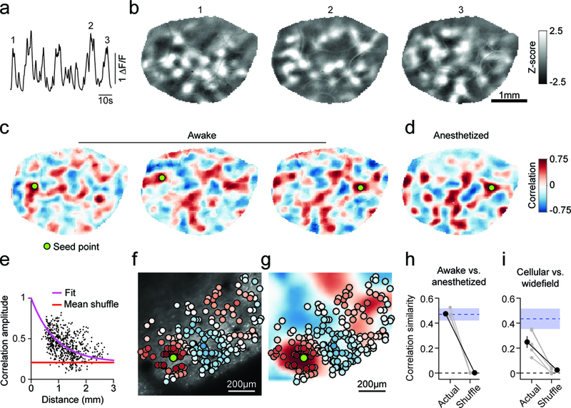
Figure 1:
Correlated spontaneous activity in awake ferret visual cortex reveals large-scale modular distributed functional networks.
a. Timecourse of spontaneous activity measured withnwide-field epifluorescence in an awake ferret (mean across pixels in ROI). b . Representative z-scored images of spontaneous events atntimes indicat...
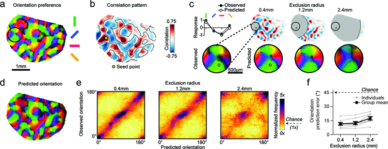
Figure 2:
Tuning properties can be predicted from correlated network elements several millimeters away.
a. Orientation preference map. b. Spontaneousncorrelation pattern (Pearsonu2019s correlation) for indicated seed point.nContour lines from vertical selective domains from ( a ) reveal thatnspontaneous...
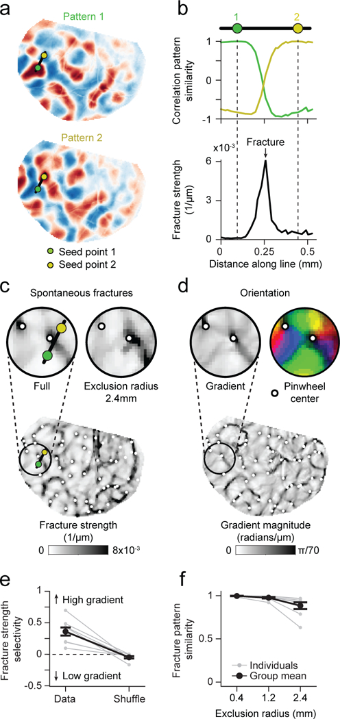
Figure 3:
Tight relation between global spontaneous correlation and fine-scale structure of orientation columns after eye-opening (EO).
a-b. Fractures in correlated networks. Advancing thenseed-point along the black line in ( a ) reveals a punctuated rapidntransition in global correlation structure expressed by a high rate of change i...
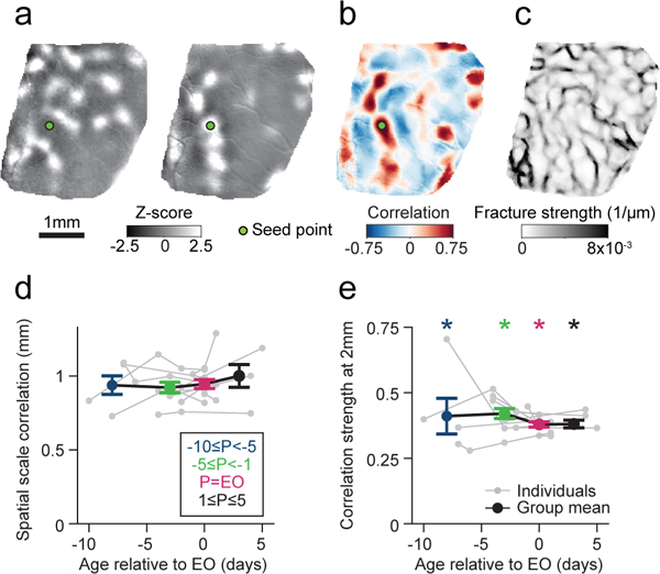
Figure 4:
Early spontaneous activity exhibits long-range correlations.
a. Representative z-scored images of early spontaneousnactivity at P23, seven days prior to EO. b-c. Early spontaneousnactivity shows hallmarks of mature spontaneous activity, including long-rangencor...
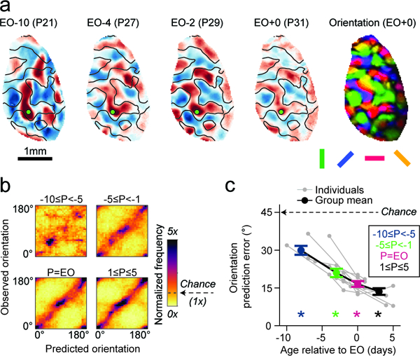
Figure 5:
Spontaneous activity prior to eye-opening predicts future evoked responses.
a. Longitudinal imaging of a chronically-implanted animalnreveals that early spontaneous correlation patterns exhibit signatures of thenmature orientation map ( right ), despite considerablenreorganiz...
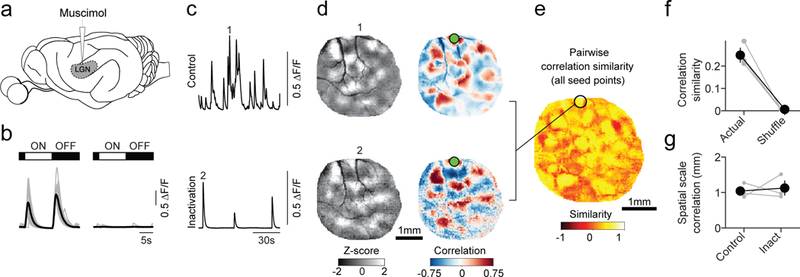
Figure 6:
Long-range correlations in spontaneous activity persist in the absence of feed-forward input.
a . Cortical spontaneous activity was measured before andnfollowing LGN inactivation via targeted muscimol infusion. b .nCortical responses (averaged across all pixels in ROI) to full-field luminancen...
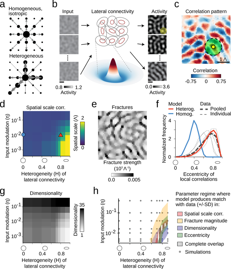
Figure 7:
Circuit mechanisms for long-range correlations in early visual cortex.
a. Homogenous local connections (arrow) induce moderatencorrelations (black dots) with all nearby domains (black dots), whereasnheterogeneity introduces biases, strengthening some correlations (large ...
Figure images are served from the NIH/NLM PubMed Central Open Access Subset or Europe PMC; copyright remains with the publishers and authors.
💬 Discussion
0 commentsNo comments yet. Be the first to start a discussion!
Leave a Comment