Abstract
During embryogenesis tissue layers undergo morphogenetic flow rearranging and folding into specific shapes. While developmental biology has identified key genes and local cellular processes, global coordination of tissue remodeling at the organ scale remains unclear. Here, we combine in toto light-sheet microscopy of the Drosophila embryo with quantitative analysis and physical modeling to relate cellular flow with the patterns of force generation during the gastrulation process. We find that the complex spatio-temporal flow pattern can be predicted from the measured meso-scale myosin density and anisotropy using a simple, effective viscous model of the tissue, achieving close to 90% accuracy with one time dependent and two constant parameters. Our analysis uncovers the importance of a) spatial modulation of myosin distribution on the scale of the embryo and b) the non-locality of its effect due to mechanical interaction of cells, demonstrating the need for the global perspective in the study of morphogenetic flow.
🔬 Techniques
🔭 Microscopes
🧬 Organisms
💻 Software
✨ Fluorophores
🧪 Sample Preparation
🔬 Cell Lines
🏭 Microscope Brands
🧪 Reagent Suppliers
🔴 Lasers
📷 Detectors
🔎 Objectives
💻 Software Details
💾 Data Repositories
🏛️ Research Organizations (ROR)
Affiliated research institutions:
📋 Methods
Fly lines used His2Av-mCherry ( Krzic et al., 2012 ), bcd e1 nos bn tsl 4 /TM3, halo twi ID96 /Cyo (twi ID96 is also known as twi [ Martin et al., 2009 ]), sqh-GFP klar ( Martin et al., 2009 ), OregonR. Embryos where dechorionated following standard procedures, and mounted in agarose gels as previously described ( Krzic et al., 2012 ).
Light sheet microscopy
Fluorescence-based live imaging was carried out on a MuVI SPIM ( Krzic et al., 2012 ). Briefly, the optics consisted of two detection and illumination arms. Each detection arm forms a water-dipping epifluorescence microscope, consisting of an objective (Apo LWD 25x, NA 1.1, Nikon Instruments Inc.), a filter wheel (HS-1032, Finger Lakes Instrumentation LLC), with emission filters (BLP01-488R-25, BLP02-561R-25, Semrock Inc.), tube lens (200 mm, Nikon Instruments Inc.), and an sCMOS camera (Zyla 4.2, Andor Technology plc.), with an effective pixel size of 0.26 µm. Each illumination arm consisted of a water-dipping objective (CFI Plan Fluor 10x, NA 0.3), a tube lens (200 mm, both Nikon Instruments Inc.), a scan lens (S4LFT0061/065, Sill optics GmbH and Co. KG), and a galvanometric scanner (6215 hr, Cambridge Technology Inc.), fed by lasers (06-MLD 488 nm, Cobolt AB, and 561LS OBIS 561 nm, Coherent Inc.). Optical sectioning is achieved by translating the sample using a linear piezo stage (P-629.1cd with E-753 controller) sample rotation is performed with a rotational piezo stage (U-628.03 with C-867 controller) and a linear actuator (M-231.17 with C-863 controller, all Physik Instrumente GmbH and Co. KG).
Show full methods section
Fly lines used His2Av-mCherry ( Krzic et al., 2012 ), bcd e1 nos bn tsl 4 /TM3, halo twi ID96 /Cyo (twi ID96 is also known as twi [ Martin et al., 2009 ]), sqh-GFP klar ( Martin et al., 2009 ), OregonR. Embryos where dechorionated following standard procedures, and mounted in agarose gels as previously described ( Krzic et al., 2012 ).
Light sheet microscopy
Fluorescence-based live imaging was carried out on a MuVI SPIM ( Krzic et al., 2012 ). Briefly, the optics consisted of two detection and illumination arms. Each detection arm forms a water-dipping epifluorescence microscope, consisting of an objective (Apo LWD 25x, NA 1.1, Nikon Instruments Inc.), a filter wheel (HS-1032, Finger Lakes Instrumentation LLC), with emission filters (BLP01-488R-25, BLP02-561R-25, Semrock Inc.), tube lens (200 mm, Nikon Instruments Inc.), and an sCMOS camera (Zyla 4.2, Andor Technology plc.), with an effective pixel size of 0.26 µm. Each illumination arm consisted of a water-dipping objective (CFI Plan Fluor 10x, NA 0.3), a tube lens (200 mm, both Nikon Instruments Inc.), a scan lens (S4LFT0061/065, Sill optics GmbH and Co. KG), and a galvanometric scanner (6215 hr, Cambridge Technology Inc.), fed by lasers (06-MLD 488 nm, Cobolt AB, and 561LS OBIS 561 nm, Coherent Inc.). Optical sectioning is achieved by translating the sample using a linear piezo stage (P-629.1cd with E-753 controller) sample rotation is performed with a rotational piezo stage (U-628.03 with C-867 controller) and a linear actuator (M-231.17 with C-863 controller, all Physik Instrumente GmbH and Co. KG).
Experiment control and data fusion
Stages and cameras are controlled using Micro Manager ( Edelstein et al., 2014 ), to coordinate time-lapse experiments, running on a Super Micro 7047GR-TF Server, with 12 Core Intel Xeon 2.5 GHz, 64 GB PC3 RAM, and hardware Raid 0 with 7 2.0 TB SATA hard drives. Samples were recorded from two, by 90 0 rotated views, at a typical optical sectioning of 1 µm, and temporal resolution of 75 s. As previously described ( Krzic et al., 2012 ), MuVI SPIM optical stability allows a fusion strategy based on a diagnostic specimen. Recorded once per experiment, the diagnostic specimen is used to determine an initial guess for an affine transformation, which we feed into a rigid image registration algorithm ( Klein et al., 2010 ), to fuse individual views, resulting in an isotropic resolution of. 26 µm in the registered image.
Surface of Interest extraction
We used tissue cartography to extract surfaces of interest (SOI) from embryos ( Heemskerk and Streichan, 2015 ). Briefly, we identify the outline of the sample using the Ilastik detector to determine a point cloud for SOI construction. In a fitting step (implemented in the sphere-like fitter), we create a smooth description of the SOI in terms of cylinder coordinates defined by AP axis and azimuth ( Heemskerk and Streichan, 2015 ). Image intensity data are then projected onto a nested group of 5 layers (two normally evolved layers above and below the SOI), each three pixels apart, defining a 3–4 µm thick 'curved image stack'. For analysis the maximum intensity projection of nested layers was used. Although the shape of embryos of the same genotype is highly reproducible, small differences in the underlying point cloud can result in small differences of the SOI passing through the apical cell surface. To simplify comparison between embryos, we create a standard projection on a cylinder grid of fixed size, with the embryo surface oriented such that apical is left, posterior right, dorsal in the center, and ventral on top and bottom ( Figure 1 ). Systematic distortions of measurements due to projecting the curved embryo surface to the plane are corrected using the metric tensor ( Heemskerk and Streichan, 2015 ). The apical surface is static, while the dynamic basal cell surface moves with the cellularization front. Projections of the latter could be created by reading signal on a surface obtained by evolving the apical SOI along its normal basal wards. However, small differences in cell height ( e m b r y o d t where < > e m b r y o denotes averaging across the embryo, v → r e f is an arbitrary chosen reference from the ensemble, and v ⃑ i , t o f f , i denote the i-th flow field and offset time respectively. In this way, we align samples to a chosen reference, in which we use the first occurrence of the cephalic furrow (CF) as a landmark indicating our choice for t = 0 min. Within a given genotype, we could automatically determine the offset time. However, to align mutants to WT, we first aligned all mutant datasets, and then used landmarks such as the CF ( twist ), or the VF ( bcd nos tsl ), to define a common time frame as best as possible. Time shifted accordingly, we created an ensemble average flow field for each genotype: < v → > e n s e m b l e : = 1 N ∑ i N v → i ( t − t o f f , i ) The magnitude of ensemble average is highly reproducible from embryo to embryo (note the small standard deviation Figure 1—figure supplement 5a ). Flow trajectories during cellularization point towards the dorsal side ( Figure 1—figure supplement 5b ), showing persistent movement towards dorsal regions during pre-CF flow. This is accompanied by reduction of apical cell area in these regions ( Figure 1—figure supplement 5c ), as measured using confocal microscopy. While the length of pre-VF flow lines peaks on the anterior and posterior poles in WT, it is substantially reduced near poles in twist , and only mildly reduced in bcd nos tsl ( Figure 1—figure supplement 5d–f ). Together with the loss of basal DV asymmetry, this suggests that twist mediated reduction of basal myosin levels on the ventral side is responsible for dorsal-ward flow.
Myosin quantification Intensity normalization
Using the imaging and pre-processing procedure as outlined above with samples expressing sqhGFP ( Royou et al., 2002 ), we created projections of the apical and basal cell surfaces, with the goal of establishing a quantitative measurement of global myosin patterns ( Figure 1—figure supplements 6 and 7 ). Ideally, quantification of signal intensities is carried out using identical conditions for each sample in the pool used for statistics, to minimize variability across samples. However, when performing in toto live-imaging, it is difficult to image more than one sample at a time and keep a high recording frequency. To minimize variability in a sequential recording scheme, we keep imaging conditions constant, but there are still possible variabilities in recorded signal intensity for biological but also technical reasons. To account for such variability between experiments, we normalize recorded data ( Figure 1—figure supplement 6b,b’,c ). Signal intensity of all time points in a given experiment are summarized by normalizing the intensity distribution: upper and lower range are determined according to the l l = 0 and u l = 95 -percentile; normalization is done by subtracting the l l and dividing by ( u l - l l ) , yielding a dimensionless normalized signal distribution (compare Figure 1—figure supplement 6b and b’ ). This strategy should not only allow for comparison on the same microscope, but also across microscopes, allowing for validation of in toto live-imaging from sequential experiments against fixed batches imaged e.g. on a confocal.
Basal myosin pool analysis via light sheet microscopy
Here, we briefly outline the results for the DV asymmetry in the basal myosin pool that we reported in the main text. First, we time align intensity normalized basal projections as described above. Next we convolve each pullback with a Gaussian of width σ ~ 3 cell diameters to obtain basal myosin at the mesoscale (see discussion in model section below for definition). The results are then ensemble averaged to obtain ensemble myosin distribution as shown in Figure 1—figure supplement 6 . To assess DV asymmetry, we focus on the region outlined by the black/white dashed line, where we first take an average along the AP axis and then compute average signal on dorsal side, and subtract from it the average signal on the ventral side. Repeating the outlined routine for all time points, we obtain the plot show in main text Figure 4b . Basal myosin pool via confocal microscopy Figure 1—figure supplement 7c shows DV cross sections of fixed embryos stained for rb anti zipper and mouse anti dorsal, cut along the AP axis, and imaged on a confocal microscope. DV orientation of the samples is automatically determined based on the dorsal signal. To estimate the age of fixed embryos in relation to live-imaging data, we constructed a calibration curve for cell apico-basal height shown in Figure 1—figure supplement 7a . Using the known monotonic relation between cell height and age ( Merrill et al., 1988 ), which we find lasts until about 8 m i n after CF formation, we obtain estimate for the age of a fixed embryo based on measuring cell height. By segmenting the outline of basal myosin, we can then measure DV asymmetry in the same way as described for live-imaging data above. A direct comparison between live imaging-based DV asymmetry measurement, and based on N = 345 fixed DV cross sections from confocal shows that after applying normalization routine as described above, we find similar estimates for the DV asymmetry using both light sheet and confocal imaging (see Figure 1—figure supplement 7b ). Note that uncertainties in the calibration curve propagate to exact age determination in the embryo, and thus increased fluctuations in DV asymmetry determined using confocal imaging.
Finite element implementation
Inversion of the continuum equation of state relating the coarse-grained myosin tensor and cellular flow-field was achieved using Finite Element Methods (FEM) in the weak formulation implemented within the FELICITY toolbox for MATLAB ( Walker, 2017 ). Equations were inverted on a static triangular mesh representing the 'canonical' embryo surface produced via a point cloud (described above) subsequently turned into a smooth triangulation using MeshLab ( Cignoni, 2008 ). As such, all objects within the equation of state had to be parameterized within the 3D embedding space of the mesh, which can be done by using the direction relation between projections and SOI ( Heemskerk and Streichan, 2015 ). The only dynamic input to this inversion algorithm is the divergence of the myosin tensor. This was computed by interpolating the gradient of each Cartesian component of the tensor onto triangular faces of our mesh, producing a 3 × 3 × 3 object on each face. The partial trace of this object over directions within the tangent plane of the face result in the estimated divergence. This operation was repeated for all myosin pools used. All equations within the FEM software are projected onto the surface of our 3D mesh to manually ensure solutions only exist within the tangent plane. To benchmark the quality of our FEM solver, we implemented the equation of motion on a sphere and tested results for known solutions, which confirmed our solver works within the expected numerical accuracy. To test dependence on discretization used, we compared our results using different meshes at varying mesh sizes, and found good agreement with all test cases. In order to model internalization of the VF, we introduced the ability to add a 'cut' within the triangular mesh. Contraction of the tissue was modeled by manually introducing local force dipoles on edges within the mesh pointing along the bond. All vertices along the cut were given zero bulk modulus to allow for local tissue compression needed to simulate invagination. The location of the cut was estimated from the PIV flow fields. Specifically the ratio of the divergence of the velocity field to the velocity field's magnitude was used to estimate the spatial extent of the cut over times during ventral furrow formation. Predictions for the flow field obtained via inversion are subject to an overall scale factor, that can't be determined by the model. To compare ensemble averaged flow field measurement v ⃑ ( t ) to model predictions u ⃑ ( t ) in a quantitative fashion, we define a global measure for the spatial residual that is insensitive to such a scale factor. With the short hand notation < u → > : = < u → ( x ) 2 > e m b r y o to define overall magnitude of the field u across the surface of the embryo ( < u → ( x ) 2 > e m b r y o denotes averaging the space dependent field u ⃑ ( x ) 2 across the embryo surface, so is not space dependent.), the residual is defined as R = ( < u → > 2 v → ( x ) 2 + u → ( x ) 2 < v → > 2 ) − 2 u → > 2 < v → > 2 v → ( x ) u → ( x ) 2 < u → > 2 < v → > 2 provides a spatial discrepancy map, indicating the prediction quality as a function of location on the embryo, that is in-sensitive to noise dominated fluctuations in domains of no flow (i.e. fixed points), as opposed to e.g. inner product.
Additional files 10.7554/eLife.27454.019 Transparent reporting form
📊 Figures
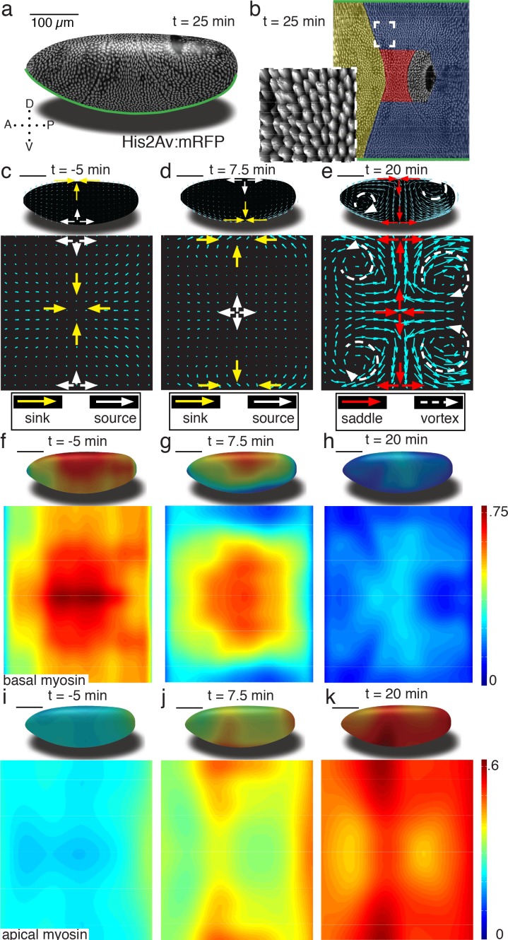
Figure 1.
Tissue deformations of Drosophila melanogaster embryos during gastrulation, captured by three simple flow fields.
( a ) Stage 7 embryo labeled with His2Av:mRFP. Anterior is to the left, dorsal up. Time is chosen such that 0 min coincides with the first occurrence of the cephalic furrow (CF). All scale bars indica...
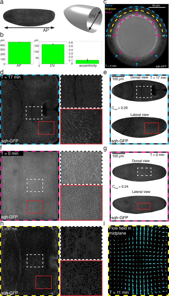
Figure 1u2014figure supplement 1.
Definition of embryo shape and relevant surfaces of interest.
( a ) D. melanogaster embryo shape characterized in terms of AP length, DV diameter, and eccentricity. ( b ) Ensemble quantification for AP length, DV diameter, and eccentricity. Error-bars indicate s...
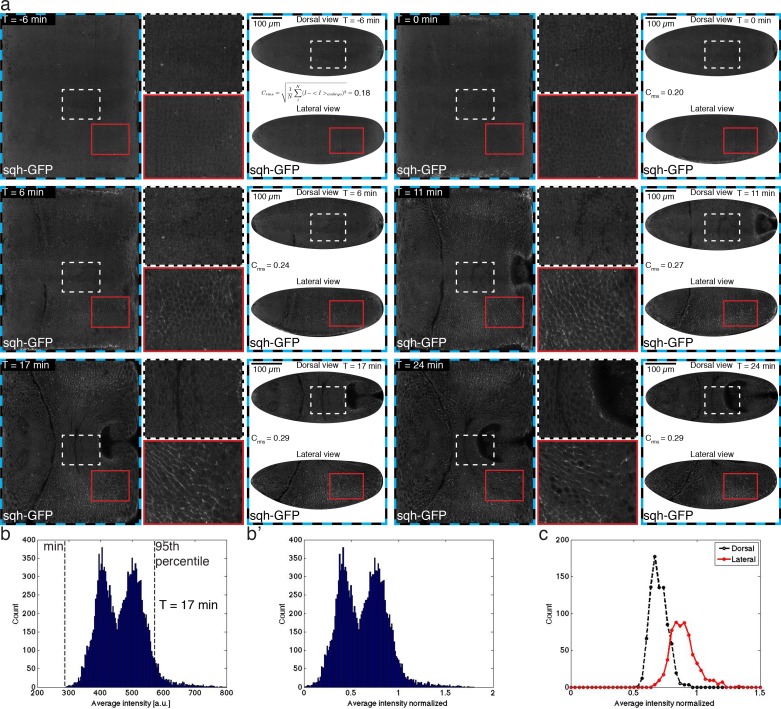
Figure 1u2014figure supplement 2.
Myosin timecourse on the apical surface.
( a ) Time course of Myosin visualized by sgh-GFP on apical surface, as described in Figure 1u2014figure supplement 1e . Root mean square contrast C rms for across the entire embryo surface is reporte...
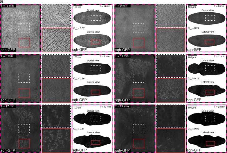
Figure 1u2014figure supplement 3.
Time course of Myosin on basal surface, as described in Figure 1u2014figure supplement 1g .
Root mean square contrast C rms for across the entire embryo surface is reported for each time point shown. Images have been normalized to range from 0 to 1 as described in the SI.
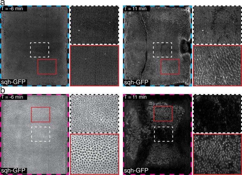
Figure 1u2014figure supplement 4.
Magnified view of time course of Myosin on basal surface, as described in Figure 1u2014figure supplement 1e,g .
( a ) apical surface. ( b ) basal surface. Note that in contrast to Figure 1u2014figure supplements 1 u2013 3 , the lookup table has been adjusted in each time point separately, to enhance visualizati...
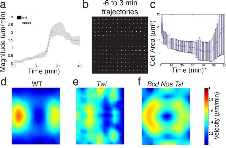
Figure 1u2014figure supplement 5.
Quantitative analysis of ensemble flow field.
( a ) WT ensemble averaged flow field magnitude, averaged over embryo surface. Standard deviation is across samples. ( b ) Flow lines obtained by integrating flow field over time, for WT embryos u2212...
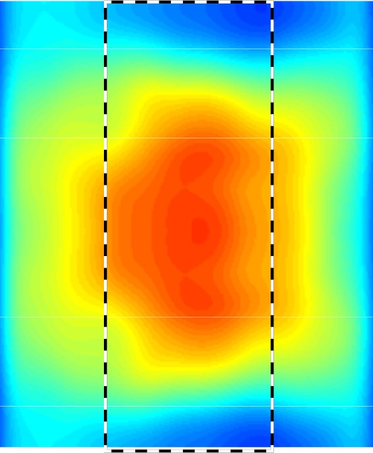
Figure 1u2014figure supplement 6.
Isotropic basal myosin, (as main text Figure 1g ).
Dashed box indicates region used to evaluate DV asymmetry.
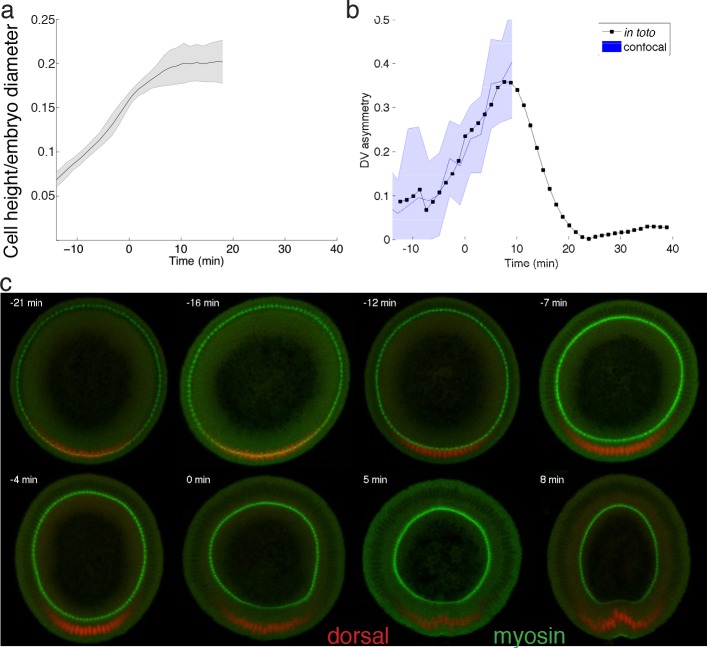
Figure 1u2014figure supplement 7.
Basal myosin quantification light sheet versus confocal.
( a ) Cell height as a function of embryo diameter increases monotonically until ventral furrow formation starts. ( b ) DV asymmetry as a function of time, measured using light sheet (black), or confo...
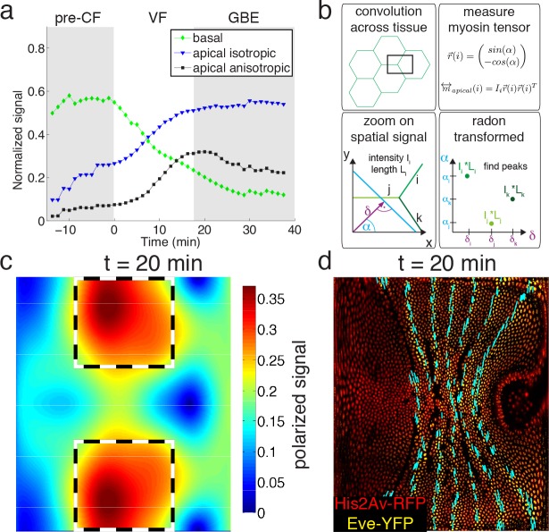
Figure 2.
Quantitative analysis of myosin distribution and anisotropy reveals transition across pools.
( a ) Normalized signal strength of basal, apical, and polarized pools over time in the lateral ectoderm (outlined as dashed box in c). First gray shaded box at tu00a0<u00a00 min indicates times be...
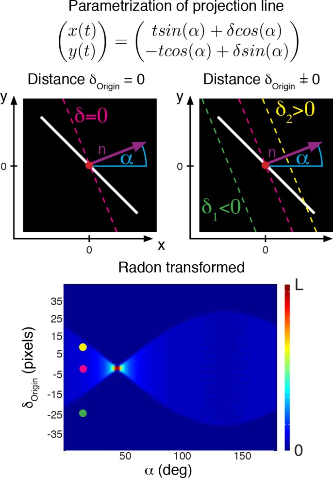
Figure 2u2014figure supplement 1.
Illustration of how to construct a Radon transform for an image with constant background I = 0 , shown in black and foreground I = 1 , shown in white (top), and resulting radon transform (bottom).
Colors indicate different lines, and the result in the radon transform is indicated as colored circle.
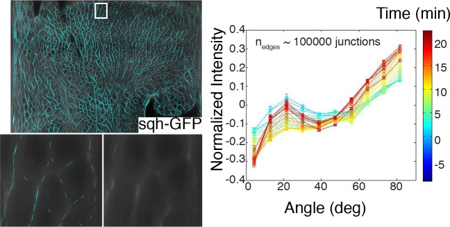
Figure 2u2014figure supplement 2.
Example of edges identified with our anisotropy detection algorithm, and a magnification in a region of interest showing result in comparison with underlying raw data (left).
Time course of normalized intensity (shifted to zero mean) versus edge orientation. Color codes for time as indicated in the colorer (right).
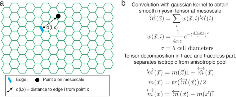
Figure 2u2014figure supplement 3.
Continuous representation of myosin tensor on the mesoscale.
( a ) Continuous representation of the myosin tensor. Black dot indicates coordinates on mesoscale and green cells represent the tissue. Edge i is highlighted in blue, and distance of edge i to a poin...
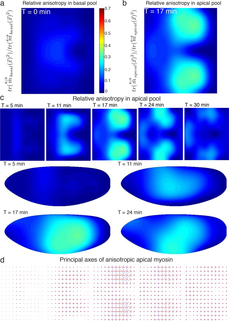
Figure 2u2014figure supplement 4.
Myosin tensor on the mesoscale.
( a ) Relative myosin anisotropy of basal pool, as computed by the magnitude of the traceless part over the total myosin tensor. ( b ) Relative myosin anisotropy of apical pool. ( c ) Time course of r...
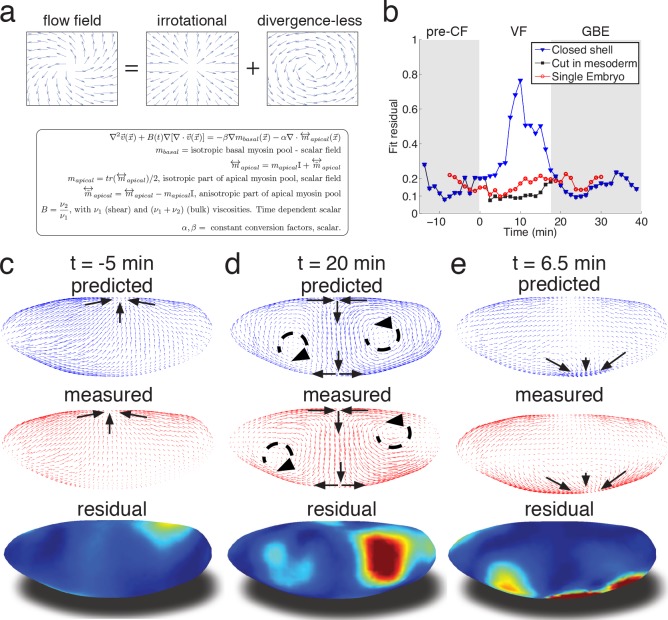
Figure 3.
Biophysical model quantitatively predicts tissue flow based on quantitative measurements of myosin distribution.
( a ) Proposed mathematical description of the flow parameterizes complex mechanics of cytoskeleton in terms of the shear u03bd 1 and u03bd 2 bulk effective viscosities. The flow is driven by the forc...
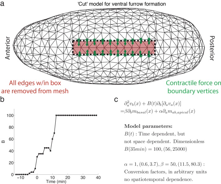
Figure 3u2014figure supplement 1.
Finite element realization of model and parameter values.
( a ) Schematic of the finite element model including the u2018cutu2019 used to model ventral furrow formation. Shown is a triangulation of the embryo from a ventral perspective, anterior to the left....
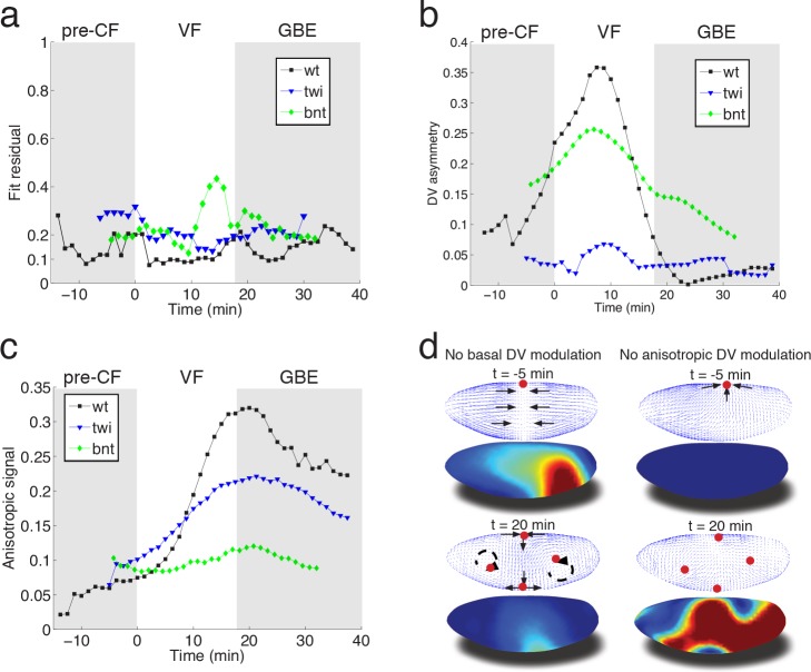
Figure 4.
Mutant analysis reveals global modifications of myosin dynamics.
( a ) Fit residual as in Figure 3b , for twi , and bcd nos tsl mutants (7, and 7 embryos in ensemble). WT is shown as reference. ( b ) Amplitude of basal myosin pool along DV axis for WT and mutants i...
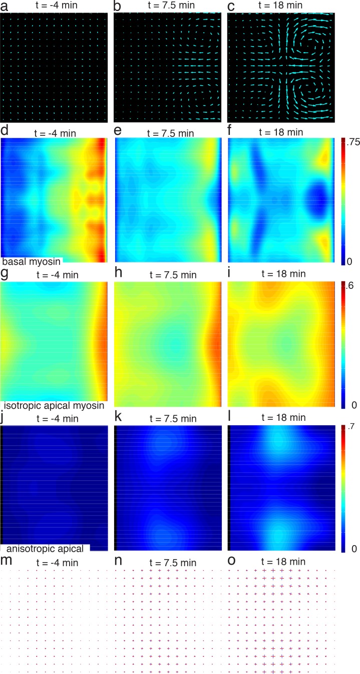
Figure 4u2014figure supplement 1.
Twist mutant flow field and myosin analysis.
( au2013c ). Flow field on 2D projections for representative time points. As in Figure 1cu2013e Cyan arrows indicate tissue flow field. ( du2013f ) Normalized myosin distribution on basal cell surface...
Figure images are served from the NIH/NLM PubMed Central Open Access Subset or Europe PMC; copyright remains with the publishers and authors.
💬 Discussion
0 commentsNo comments yet. Be the first to start a discussion!
Leave a Comment