Abstract
Abstract Brillouin microscopy can assess mechanical properties of biological samples in a three-dimensional (3D), all-optical and hence non-contact fashion, but its weak signals often lead to long imaging times and require an illumination dosage harmful for living organisms. Here, we present a high-resolution line-scanning Brillouin microscope for multiplexed and hence fast 3D imaging of dynamic biological processes with low phototoxicity. The improved background suppression and resolution, in combination with fluorescence light-sheet imaging, enables the visualization of the mechanical properties of cells and tissues over space and time in living organism models such as fruit flies, ascidians and mouse embryos.
🔬 Techniques
🧬 Organisms
💻 Software
✨ Fluorophores
🧪 Sample Preparation
🔬 Cell Lines
🏭 Microscope Brands
🧪 Reagent Suppliers
📷 Detectors
🎨 Filters
💻 Software Details
💾 Data Repositories
🏛️ Research Organizations (ROR)
Affiliated research institutions:
📋 Methods
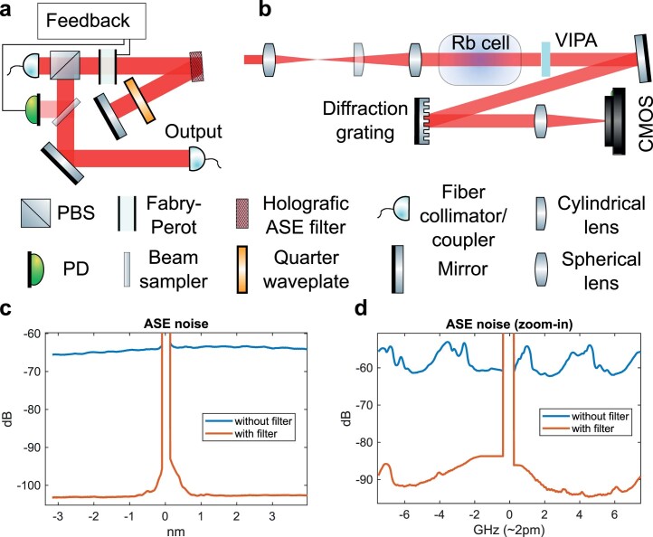
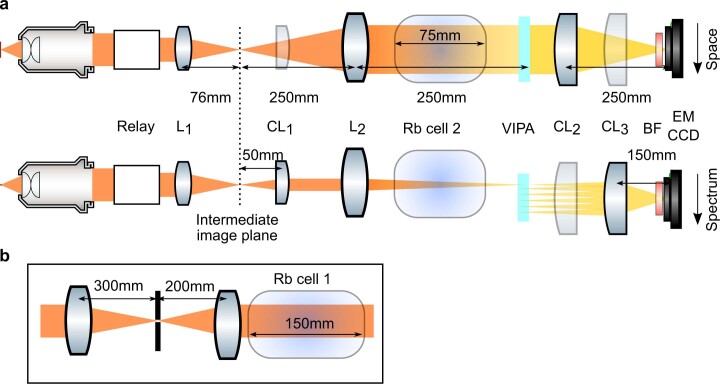
Line-scan Brillouin imaging set-up A detailed schematic diagram of our LSBM is shown in Extended Data Fig. 1 . The laser is an amplified tunable diode laser (TA pro, Toptica) locked to the D 2 , F = 2 absorption line of 87 Rb (780.24 nm). To clean the laser’s spectrum to remove amplified spontaneous emission (ASE) noise, we designed a custom-built narrowband double-pass optical filter 32 , consisting of a polarizing beam splitter followed by a tunable Fabry–Pérot cavity (free spectral range (FSR) 15 GHz, Finesse ~60, LightMachinery), a holographic diffraction grating (NoiseBlock, Coherent), a quarter waveplate and a mirror. A beam sampler (BSF10-B, Thorlabs) sends ~5% of the light to a photodiode, the signal from which is fed into Arduino Uno SMD R2 and PmodDA3 digital to analog converter boards; a self-written Arduino 1.8.13 code maximizes the transmitted intensity to correct for long-term drift of the cavity (Extended Data Fig. 2a ). The filter enables a total suppression of the integrated ASE noise down to approximately −90dB, more than 40 dB below the original ASE level of the laser (Extended Data Fig. 2c ). After the filter, the light is coupled into a polarization-maintaining fiber and delivered to the main microscope. Here, a collimator (LPC-OT-780-5/125-P-3-16AC-40-3A, OZ Optics) produces a collimated beam with a diameter of 2.77 mm (1/e 2 , theoretical), which corresponds to a focused beam of 1.79 µm (1/e 2 , theoretical) after the objective. The beam then passes through an electrically tunable lens (EL-10-30, Optotune) coupled with a negative offset lens (LC1258-B, Thorlabs). This enables axial scanning of the focus position after the objective (Extended Data Fig. 6 ). After the tunable lens, a flip mirror enables switching between the epi-line and orthogonal-line illumination: the separate optical path for the epi-line illumination consists of a 40 mm lens (LA1422-B, Thorlabs) that collimates the light out of a polarization-maintaining fiber (P3-780PM-FC-2, Thorlabs) to provide a beam of diameter 8.7 mm (1/e 2 , theoretical) (filling the back focal aperture of the objective, which is 8 mm); a 200 mm cylindrical lens (LJ1653RM-B, Thorlabs) generates the focused line in the focal plane of the objective with an extension of ~185 µm (1/e 2 ) (Extended Data Fig. 6 ). A half waveplate (WPH05M-780, Thorlabs) is used to rotate the linear polarization of the illumination light to match the required direction for the two geometries. Two mirrors, conjugated to the back and the front focal plane of the objective (by means of two 200 m lenses: cat. nos. 33-362 and 49-364, Edmund), respectively, enable fine position and angle adjustment of the beam inside the sample to aid in the alignment between the illumination and detection objectives. For the fluorescence SPIM modality, we use a laser box providing several laser lines for fluorescence excitation (405 nm, 488 nm, 560 nm, 640 nm). The fluorescence excitation is introduced into the set-up by a single mode fiber (P1-460Y-FC-1, Thorlabs), the output of which is collimated by an achromatic lens (f = 4 mm), to produce an ~0.8 mm (1/e 2 , theoretical) beam. A fiber polarization controller (FPC030, Thorlabs) is used to adjust the polarization and a polarizer rejects potential residual non-linear polarization. The excitation light is then coupled into the same optical path as the Brillouin illumination by means of a dichroic mirror (FF765-Di01, Semrock). Similarly to the Brillouin illumination path, two lenses (67-159, Edmund and 49-364, Edmund, shared with the Brillouin path) and mirrors (not shown in Extended Data Fig. 1 ) enable beam adjustment. An 18 mm cylindrical lens (68-041, Edmund) is used to generate the light sheet. The corresponding thickness and lateral extent of the light sheet inside the sample are ~4 µm and ~200 µm (1/e 2 , theoretical), respectively. The detection and illumination objectives are identical (Nikon, ×40, 0.8 numerical aperture, MRD07420, water immersion) and oriented in an inverted V configuration to facilitate the imaging of small (~200 µm) samples in physiological conditions 21 (Fig. 1a and Extended Data Fig. 1 ). The sample is placed in a dedicated, custom-built chamber that utilizes a 12.7-µm-thick fluorinated ethylene propylene (FEP) foil (RD-FEP050A-610, Lohmann) to separate the immersion water of the objectives from the sample. The sample’s environment (medium) is temperature controlled via a custom-built heating element and PID (proportional–integral–derivative) controller, and CO 2 is added via a custom-built gas-mixer (Extended Data Fig. 1c,d ). For 3D image acquisition, the chamber containing the sample is scanned by three single-axis translational stages (SLC-2430, SmarAct). For the epi-line Brillouin geometry (E-LSBM), a polarizing beam splitter (BPB-12.7SF2-R400-800, Lambda), mounted on a magnetic base for easy switching between the two modalities, followed by a quarter waveplate (WPRM-25.4-12.7CQ-M-4-780, Lambda), reflects the light towards one of the two objectives; the Brillouin signal is collected by the same objective and transmitted by the polarizing beam splitter towards the spectrometer (the polarization is rotated by 90° due to the double pass at the quarter waveplate). A polarizer is added before the other objective (used for SPIM excitation), which is required to block the backwards-scattered un-polarized fluorescence light that would otherwise be reflected by the polarizing beam splitter, and generate a bright line at the center on the FOV of the SPIM camera. The fluorescence and Brillouin signals are split via a dichroic mirror (FF765-Di01, Semrock), reflecting the fluorescence emission. A tube lens (MXA20696, Nikon) focuses the fluorescence image on the SPIM camera (Zyla sCMOS, Andor); a motorized filter wheel (96A361, Ludl) enables selection of the proper emission filter. The Brillouin signal is instead transmitted by the dichroic mirror and sent to the spectrometer (Extended Data Fig. 3 ). Here, first two spherical lenses (LA1256-B and LA1979-B-ML, Thorlabs) relay the back focal aperture of the detection objective and a slit (VA100/M, Thorlabs), placed in the focal plane of the first lens, ensures confocality in the direction perpendicular to the illumination line. After the relay, inelastically scattered (Rayleigh) light is filtered by a 150-mm-long gas cell filled with pure 87 Rb (SC-RB87-(25×150-Q)-AR, Photonics Technologies). The cell is wrapped into heating foil (HT10K, Thorlabs) and a self-built electronic board (based on an Arduino Mega) controls the temperature of the cell via PID. After the rubidium gas cell, a combination of an achromatic lens (cat. no. 49-794, Edmund), a cylindrical lens (cat. no. 36-231, Edmund) and a spherical lens (cat. no. 69-513, Edmund) relay and focus the light onto the entrance slit of the virtually imaged phased array (VIPA; OP-6721-6743-9, LightMachinery). Between the second spherical lens and the VIPA there is an additional 75-mm-long 87 Rb cell (SC-RB87-(25×75-Q)-AR, Photonics Technologies). After the VIPA two cylindrical lenses (LJ1267L1-B and LJ1629L2-B, Thorlabs) focus the light on the EMCCD (electron-multiplying charge-coupled device) camera (iXon DU-897U-CS0-BV, Andor), preceded by a bandpass filter (FBH780-10, Thorlabs) to block ambient light. These lenses are chosen to ensure proper spatial and spectral sampling (0.7 µm px −1 and ~0.25 to ~0.5 GHz px −1 ). The optical layout and performance are shown in Extended Data Figs. 3 – 5 . To synchronize the electrically tunable lens with the EMCCD acquisition, the fire output of the EMCCD (high when the camera is exposing) is used to trigger a data acquisition device (PCI-6221, National Instruments) that generates the voltage ramp driving the electrically tunable lens. The entire data acquisition is controlled by a self-written LabView2018 program and the image reconstruction is performed with a Matlab2018 script, which provides an interface to the GPU-fitting library (see the section Brillouin line-scan spectral analysis ).
Show full methods section
Line-scan Brillouin imaging set-up A detailed schematic diagram of our LSBM is shown in Extended Data Fig. 1 . The laser is an amplified tunable diode laser (TA pro, Toptica) locked to the D 2 , F = 2 absorption line of 87 Rb (780.24 nm). To clean the laser’s spectrum to remove amplified spontaneous emission (ASE) noise, we designed a custom-built narrowband double-pass optical filter 32 , consisting of a polarizing beam splitter followed by a tunable Fabry–Pérot cavity (free spectral range (FSR) 15 GHz, Finesse ~60, LightMachinery), a holographic diffraction grating (NoiseBlock, Coherent), a quarter waveplate and a mirror. A beam sampler (BSF10-B, Thorlabs) sends ~5% of the light to a photodiode, the signal from which is fed into Arduino Uno SMD R2 and PmodDA3 digital to analog converter boards; a self-written Arduino 1.8.13 code maximizes the transmitted intensity to correct for long-term drift of the cavity (Extended Data Fig. 2a ). The filter enables a total suppression of the integrated ASE noise down to approximately −90dB, more than 40 dB below the original ASE level of the laser (Extended Data Fig. 2c ). After the filter, the light is coupled into a polarization-maintaining fiber and delivered to the main microscope. Here, a collimator (LPC-OT-780-5/125-P-3-16AC-40-3A, OZ Optics) produces a collimated beam with a diameter of 2.77 mm (1/e 2 , theoretical), which corresponds to a focused beam of 1.79 µm (1/e 2 , theoretical) after the objective. The beam then passes through an electrically tunable lens (EL-10-30, Optotune) coupled with a negative offset lens (LC1258-B, Thorlabs). This enables axial scanning of the focus position after the objective (Extended Data Fig. 6 ). After the tunable lens, a flip mirror enables switching between the epi-line and orthogonal-line illumination: the separate optical path for the epi-line illumination consists of a 40 mm lens (LA1422-B, Thorlabs) that collimates the light out of a polarization-maintaining fiber (P3-780PM-FC-2, Thorlabs) to provide a beam of diameter 8.7 mm (1/e 2 , theoretical) (filling the back focal aperture of the objective, which is 8 mm); a 200 mm cylindrical lens (LJ1653RM-B, Thorlabs) generates the focused line in the focal plane of the objective with an extension of ~185 µm (1/e 2 ) (Extended Data Fig. 6 ). A half waveplate (WPH05M-780, Thorlabs) is used to rotate the linear polarization of the illumination light to match the required direction for the two geometries. Two mirrors, conjugated to the back and the front focal plane of the objective (by means of two 200 m lenses: cat. nos. 33-362 and 49-364, Edmund), respectively, enable fine position and angle adjustment of the beam inside the sample to aid in the alignment between the illumination and detection objectives. For the fluorescence SPIM modality, we use a laser box providing several laser lines for fluorescence excitation (405 nm, 488 nm, 560 nm, 640 nm). The fluorescence excitation is introduced into the set-up by a single mode fiber (P1-460Y-FC-1, Thorlabs), the output of which is collimated by an achromatic lens (f = 4 mm), to produce an ~0.8 mm (1/e 2 , theoretical) beam. A fiber polarization controller (FPC030, Thorlabs) is used to adjust the polarization and a polarizer rejects potential residual non-linear polarization. The excitation light is then coupled into the same optical path as the Brillouin illumination by means of a dichroic mirror (FF765-Di01, Semrock). Similarly to the Brillouin illumination path, two lenses (67-159, Edmund and 49-364, Edmund, shared with the Brillouin path) and mirrors (not shown in Extended Data Fig. 1 ) enable beam adjustment. An 18 mm cylindrical lens (68-041, Edmund) is used to generate the light sheet. The corresponding thickness and lateral extent of the light sheet inside the sample are ~4 µm and ~200 µm (1/e 2 , theoretical), respectively. The detection and illumination objectives are identical (Nikon, ×40, 0.8 numerical aperture, MRD07420, water immersion) and oriented in an inverted V configuration to facilitate the imaging of small (~200 µm) samples in physiological conditions 21 (Fig. 1a and Extended Data Fig. 1 ). The sample is placed in a dedicated, custom-built chamber that utilizes a 12.7-µm-thick fluorinated ethylene propylene (FEP) foil (RD-FEP050A-610, Lohmann) to separate the immersion water of the objectives from the sample. The sample’s environment (medium) is temperature controlled via a custom-built heating element and PID (proportional–integral–derivative) controller, and CO 2 is added via a custom-built gas-mixer (Extended Data Fig. 1c,d ). For 3D image acquisition, the chamber containing the sample is scanned by three single-axis translational stages (SLC-2430, SmarAct). For the epi-line Brillouin geometry (E-LSBM), a polarizing beam splitter (BPB-12.7SF2-R400-800, Lambda), mounted on a magnetic base for easy switching between the two modalities, followed by a quarter waveplate (WPRM-25.4-12.7CQ-M-4-780, Lambda), reflects the light towards one of the two objectives; the Brillouin signal is collected by the same objective and transmitted by the polarizing beam splitter towards the spectrometer (the polarization is rotated by 90° due to the double pass at the quarter waveplate). A polarizer is added before the other objective (used for SPIM excitation), which is required to block the backwards-scattered un-polarized fluorescence light that would otherwise be reflected by the polarizing beam splitter, and generate a bright line at the center on the FOV of the SPIM camera. The fluorescence and Brillouin signals are split via a dichroic mirror (FF765-Di01, Semrock), reflecting the fluorescence emission. A tube lens (MXA20696, Nikon) focuses the fluorescence image on the SPIM camera (Zyla sCMOS, Andor); a motorized filter wheel (96A361, Ludl) enables selection of the proper emission filter. The Brillouin signal is instead transmitted by the dichroic mirror and sent to the spectrometer (Extended Data Fig. 3 ). Here, first two spherical lenses (LA1256-B and LA1979-B-ML, Thorlabs) relay the back focal aperture of the detection objective and a slit (VA100/M, Thorlabs), placed in the focal plane of the first lens, ensures confocality in the direction perpendicular to the illumination line. After the relay, inelastically scattered (Rayleigh) light is filtered by a 150-mm-long gas cell filled with pure 87 Rb (SC-RB87-(25×150-Q)-AR, Photonics Technologies). The cell is wrapped into heating foil (HT10K, Thorlabs) and a self-built electronic board (based on an Arduino Mega) controls the temperature of the cell via PID. After the rubidium gas cell, a combination of an achromatic lens (cat. no. 49-794, Edmund), a cylindrical lens (cat. no. 36-231, Edmund) and a spherical lens (cat. no. 69-513, Edmund) relay and focus the light onto the entrance slit of the virtually imaged phased array (VIPA; OP-6721-6743-9, LightMachinery). Between the second spherical lens and the VIPA there is an additional 75-mm-long 87 Rb cell (SC-RB87-(25×75-Q)-AR, Photonics Technologies). After the VIPA two cylindrical lenses (LJ1267L1-B and LJ1629L2-B, Thorlabs) focus the light on the EMCCD (electron-multiplying charge-coupled device) camera (iXon DU-897U-CS0-BV, Andor), preceded by a bandpass filter (FBH780-10, Thorlabs) to block ambient light. These lenses are chosen to ensure proper spatial and spectral sampling (0.7 µm px −1 and ~0.25 to ~0.5 GHz px −1 ). The optical layout and performance are shown in Extended Data Figs. 3 – 5 . To synchronize the electrically tunable lens with the EMCCD acquisition, the fire output of the EMCCD (high when the camera is exposing) is used to trigger a data acquisition device (PCI-6221, National Instruments) that generates the voltage ramp driving the electrically tunable lens. The entire data acquisition is controlled by a self-written LabView2018 program and the image reconstruction is performed with a Matlab2018 script, which provides an interface to the GPU-fitting library (see the section Brillouin line-scan spectral analysis ).
LSBM system characterization and image acquisition
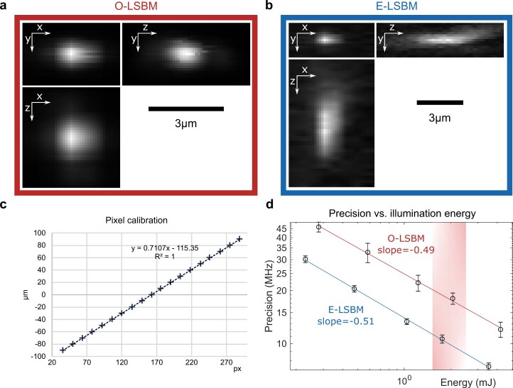
To quantify the optical resolution of the O-LSBM and E-LSBM modalities, we embedded 0.3 µm fluorescent beads (TetraSpeck, Thermo Fischer) in 1% agarose and recorded the Brillouin spectrum while scanning the sample along the y direction with a step size of 0.1 µm for O-LSBM and E-LSBM, and along the z direction with a step size of 0.1 µm for O-LSBM and 0.25 µm for E-LSBM. By assigning the amplitude of the Rayleigh peak to the corresponding spatial position, Extended Data Fig. 4a and Extended Data Fig. 4b were generated for the O-LSBM and E-LSBM modalities, respectively. The plots in Fig. 1e were generated by summing the intensity in Extended Data Fig. 4a,b along the direction perpendicular to the one shown. To quantify the spatial pixel size we moved the bead along x and performed a linear fit (Extended Data Fig. 4c ). To quantify the spectral precision we collected 50 spectrometer images (lines) from water in typical imaging conditions (100 ms integration time, less than ~18 mW), selected the spectra from the center of the FOV (where the intensity is approximately constant), determined the Brillouin shift after applying the reconstruction pipeline, and calculated the histogram (Fig. 1f ) and the standard deviation, To measure the spectrometer’s spectral resolution, we collected the Brillouin signal from scattering intralipid solution, remapped and summed the spectra (see the section Brillouin line-scan spectral analysis ) and performed a Lorentzian fit on the Rayleigh signal. The signal-to-noise ratio in a biological sample (Extended Data Fig. 10 ) was calculated as the ratio of the amplitude of the Stokes peak divided by the standard deviation of the residuals after fitting the spectra with the appropriate function (that is, the difference between the raw data and the fit). The ASE was measured with the set-up shown in Extended Data Fig. 2b , which consists of the addition of a diffraction grating to the Brillouin spectrometer to ensure an extended FSR while retaining high spectral resolution. The rubidium cells suppress the laser light, thus allowing for the very high dynamic range (>90 dB) needed for these measurements.
Brillouin line-scan spectral analysis
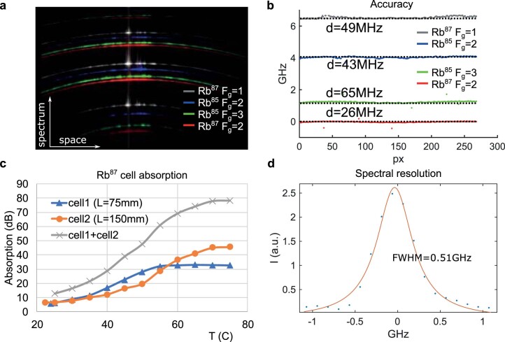
Each spectral line (corresponding to the light scattered from a point along the illumination line) is analyzed separately. The processing of this spectral data is then done in three main steps. First, the spectrum is remapped into a linear frequency space; second, the signal from at least three different orders is summed to increase the effective signal-to-noise ratio; and last, the Stokes and anti-Stokes peaks are fitted separately. To speed up the entire processing via parallelization, we decided to implement this analysis pipeline with custom GPU code written in CUDA. The linear remapping (pixel-to-frequency conversion) depends only on the position of the Rayleigh peak and the FSR of the VIPA (15.15 GHz). Here, the FSR was measured from the calibration of the spectrometer with rubidium D 2 hyperfine lines of known frequency (Extended Data Fig. 5a,b ). For the remapping we use spline interpolation whenever the target frequency sampling does not match the frequencies of individual pixels. Each line of the image can be processed independently, enabling this operation to be executed in parallel on the GPU. After this pre-processing step, the individual spectra are fitted over a user-selected range using GPUfit 33 . Lorentzian, quadratic and broadened Brillouin line shape 25 functions were custom added into this library. In addition to the main Brillouin peak position and linewidth, other fitting parameters, such as amplitude, signal-to-noise ratio, goodness of fit, and number of iterations can be retrieved. The reported Brillouin shift is the average between the frequency shift of the Stokes and anti-Stokes peaks. To benchmark our GPU pipeline, we created a synthetic Brillouin spectral signal, which we then processed with either the standard, CPU-based Matlab script or our custom GPU code. On our personal computer (Intel Core i9-11900K, 64 GB RAM and Nvidia GeForce GTX 1050 Ti), the GPU processing took ~10 ms regardless of the dimension of the image, while the purely Matlab-based pipeline took more than ~1 s, and scaled linearly with the image size (Extended Data Fig. 7a ). Both processing methods give similar results, with negligible (~1 MHz) difference between the fitted peak frequencies and the real value (Extended Data Fig. 7b ).
Drosophila embryo imaging Live imaging
Drosophila live imaging was performed with embryos expressing Gap43::mCherry to label cell membranes and EB1-GFP to mark microtubules plus ends 34 . Embryos for Brillouin imaging were prepared as follows: 1 h synchronized egg collections were performed at 25 °C and embryos were allowed to develop for a further 1 h at 25 °C. Next, halocarbon oil (27S, Sigma) was added on the agar plate carrying the collected embryos to enable accurate embryonic staging through visual inspection of morphological features under a binocular microscope (Zeiss). Embryos in stage 5a-b 35 were hand-selected, dechorionated in sodium hypochlorite (standard bleach, 50% in H 2 O) for 90 s, and washed using PBS 1X. Finally, embryos were glued (with heptane glue) to the outer surface of the FEP film in the desired orientations to enable the collection of data from different angles. Image acquisition was initiated 5 min after the cellularizing front of the blastoderm cells passed the basal side of the nuclei. The temperature of the imaging chamber was set to 22 °C.
Drosophila Snail antibody generation
A construct encoding an amino-terminal glutathione S-transferase (GST)-tagged portion of the Drosophila Snail protein (encompassing amino acids 1–200 of Uniprot ID P08044 ) was expressed in Escherichia coli and purified from lysates of bacteria expressing the Snail–GST fusion protein using beads with immobilized glutathione. The fusion protein was eluted from beads using reduced glutathione and used for immunizing a rabbit. The immunization and collection of pre-bleeds and test bleeds was performed by Cocalico Biologicals. The antiserum was tested for specificity and titer using immunostaining, immunoprecipitation and western blot analysis.
Immunohistochemistry
Drosophila whole mount embryos were fixed and stained as previously described 36 . In Fig. 2a,e , Gap43-mCherry transgenic embryos were stained using an mCherry antiserum (rabbit, 1:1,000, Abcam ab167453). In Fig. 2b , w 1118 embryos were co-stained with the anti-Snail antibody described above (Rabbit, 1:500) and an anti-disks large antibody to label the lateral membrane of cells (mouse, 1:50, 4F3, DSHB). Physical cross-sections across half of the embryonic length were produced on these stained embryos as previously described 37 . Image processing and automated image analysis To enable SPIM fluorescence image-guided analysis, the Brillouin time-lapse images were first re-scaled (bilinear interpolation) in the x and y directions using a factor of 2.5138 to match them to the dimensions of the fluorescence images. The fluorescence time-lapse was manually aligned with the Brillouin time-lapse in the y direction using half the diameter of the fluorescence image (450 pixels), and in the x direction using the co-localization of the furrow as the landmark (either the VFF or PMI furrow). The aligned fluorescent time-lapse was cropped using the Brillouin dimensions to stack the two time-lapses and produce an overlay image. For VFF image processing and quantification, for each analyzed embryo the overlaid time-lapse was re-sliced and three median projections of two slices each were used as embryonic replicates. To conduct the automated image analysis, we manually generated masks that included an 18-cell domain containing the mesoderm (Fig. 2b , late cellularization, Snail-positive cells). The region enclosed by the mask was determined by taking nine cells in each direction (left and right) from the center of the furrow. These masks were loaded by a Matlab script that filtered the Brillouin shift maps in each corresponding timepoint for each replicate and for each embryo. The average Brillouin shift in the filtered, potential mesodermal, domain and the corresponding standard deviation were calculated per embryo and plotted against time, taking time = 0 as the first sign of apical constriction. Image quantification was performed for three independent embryos undergoing VFF.
Statistical analysis
Prior to selection of the statistical test, we tested for normality using a Shapiro–Wilk test and Q-Q plot; if normality was not rejected, then parametric tests were used. To assess the statistical significance of the differences of the Brillouin shift in Fig. 2d , the average Brillouin shift in the segmented domain for the three independent embryos at timepoints −8.6 min, 0 min and 15.1 min was analyzed using a paired one-way ANOVA, followed by a post-hoc multiple comparison test (corrected for false discovery rate, using the two-stage step-up method of Benjamini, Krieger and Yekutieli, q-value = 0.1). Sphericity was not assumed (equal variability of differences). Statistical significance was set at α = 0.05. To analyze the statistical significance of the Brillouin shifts in Fig. 3h , we compared the medians between the segmented cell populations using a Friedman test. Statistical analyses were performed using Prism GraphPad v8-9.
Phallusia imaging
Live imaging Adult Phallusia mammillata were provided by the Roscoff Marine Biological Station (France) and kept at 17 °C under constant illumination. In vitro fertilized embryos were prepared as described previously 38 . Individual membranes were labeled with and imaged in artificial seawater with 5 μg ml −1 lipophilic dye FM4-64 (Invitrogen). The imaging chamber of our LSBM system was kept at 12 °C and 17 °C, respectively, in Fig. 3a,b and Fig. 3e–g .
Image data analysis
The registration of the SPIM and Brillouin images for analysis was done similarly to that for the Drosophila embryo, that is, the Brillouin image was upscaled (bilinear interpolation) to match the pixel size of the fluorescence image. A rectangular area of the same size as the Brillouin image was manually aligned around the center of the fluorescence image (using the edges of the embryo, visible in both modalities, as a guide) to match the Brillouin image. The boundaries of different tissue types were manually drawn, slice by slice, by looking at the morphology of the cells in the fluorescence image. The segmentation masks were then imported into Matlab and used to generate the plot in Fig. 3h .
Mouse embryo imaging Recovery and culture
Animal work was performed in the animal facility at the European Molecular Biology Laboratory, with permission from the institutional committee for animal welfare and institutional animal care and use (IACUC), under protocol number 2020-01-06RP. The animal facilities are operated according to international animal welfare rules (Federation for Laboratory Animal Science Associations guidelines and recommendations). (C57BL/6xC3H) F1 mice from 8 weeks of age onwards were used. Embryos were recovered from superovulated female mice mated with male mice. Superovulation was induced by i.p. injection of 5 IU pregnant mare’s serum gonadotropin (Intervet Intergonan), followed by i.p. injection of 5 IU human chorionic gonadotropin (Intervet Ovogest 1500) 44–48 h later.
Imaging
The sample holder was covered with pre-equilibrated (5 % CO 2 , 37 °C) G-1 Plus medium (~30 μl) and covered with pre-equilibrated Ovoil (~150 μl). Pockets were cast into the membrane as previously described 39 . Embryos were then mounted into the pockets for imaging.
Immunofluorescence staining
Embryos were washed twice with PBS, fixed using 1% PFA and 0.1% Triton X-100 (Sigma, T8787) in PBS for 30 min at room temperature, and then washed again three times with PBS. All these steps were carried out in IBIDI slides coated with 0.5% Agar. After washing, the embryos were transferred to uncoated IBIDI slides containing blocking buffer (PBS with 0.1% Triton X-100, 3% BSA (Sigma, 9647) and 5% normal goat serum) and incubated overnight at 4 °C. After blocking, the embryos were incubated overnight at 4 °C with primary antibodies diluted in blocking buffer. Afterwards, the embryos were washed once with 0.1% BSA and 0.1% Triton X-100 in PBS, incubated for 1 h at room temperature with secondary antibodies and DAPI (Invitrogen, D3751; 1:2,000) diluted in blocking buffer, and washed again with 0.1% BSA and 0.1% Triton X-100 in PBS. Finally, the embryos were mounted individually in 0.5 μl drops of 0.1% BSA in PBS and placed in LabTek chambers covered with oil. Primary antibodies against CDX2 (Biogenex, NC9471689; 1:150), SOX2 (Sigma, SAB3500187; 1:50) were used in this study. For the secondary staining, antibodies targeting mouse immunoglobulin coupled to Alexa Fluor 488 (Life Technologies, A21202 ), Alexa Fluor 555 (Life Technologies, A31570 ), and rabbit immunoglobulin-coupled Alexa Fluor 546 (Invitrogen, A10040 ) were used. Finally, Alexa Fluor 633-coupled phalloidin (Invitrogen, R415; 1:50) was used to stain filamentous actin. An overview of all imaging parameters used during the LSBM imaging of flies, ascidians and mouse embryos is given in Supplementary Table 1 . Reporting summary Further information on research design is available in the Nature Portfolio Reporting Summary linked to this article.
Online content Any methods, additional references, Nature Portfolio reporting summaries, source data, extended data, supplementary information, acknowledgements, peer review information; details of author contributions and competing interests; and statements of data and code availability are available at 10.1038/s41592-023-01822-1.
Supplementary information Supplementary Information Supplementary Note 1, Supplementary Table 1, Supplementary Fig. 1 and Supplementary References. Reporting Summary Peer Review File Supplementary Video 1 Brillouin shift map and fluorescence time-lapse from a Drosophila embryo undergoing ventral furrow formation (VFF).
Time-lapse of a transgenic Drosophila embryo expressing
Gap43-mCherry to fluorescently label membranes, acquired from the onset of ventral furrow formation until completion of invagination of the mesoderm. Both fluorescent and Brillouin channels were re-sliced (left, bilinear interpolation), and the resulting images were median-projected (two slices). The initiation of apical constriction was set as timepoint 0 min. The total volume of ~22 µm × 180 µm × 71 µm was acquired in ~2 min with a pixel size of 0.7 µm × 1.5 µm × 1.5 µm. Note that the acquisition of the data shown in the video required
📊 Figures
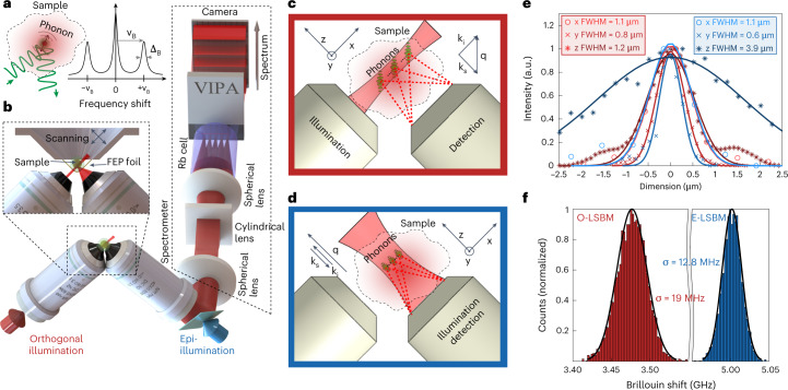
Fig. 1
Schematics and characterization of the LSBM.
a , Principle of Brillouin scattering: a small portion of the incident laser light is scattered by spontaneous thermal-induced sound waves (phonons) and gives rise to the Brillouin spectrum. b , LSBM ...
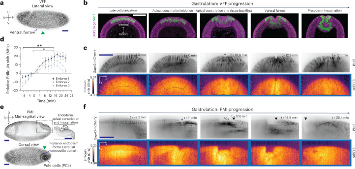
Fig. 2
Cells undergoing tissue-folding events during Drosophila gastrulation show high Brillouin shifts.
a , Surface view of a fixed Drosophila embryo undergoing VFF (arrow). The embryo expresses the membrane marker Gap43-mCherry to visualize cell outlines. The green arrowhead indicates the direction of ...
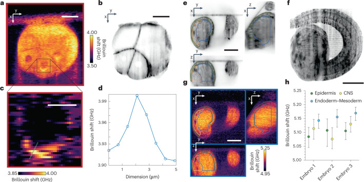
Fig. 3
LSBM imaging of Phallusia mammillata shows 3D mechanical differences on a subcellular scale and between tissue types over large volumes.
a , b , Representative O-LSBM image ( a ) and corresponding SPIM image ( b ) (membranes labeled with lipophilic dye FM4-64) of a Phallusia mammillata embryo at the 16-cell stage (out of n =u20092 in t...
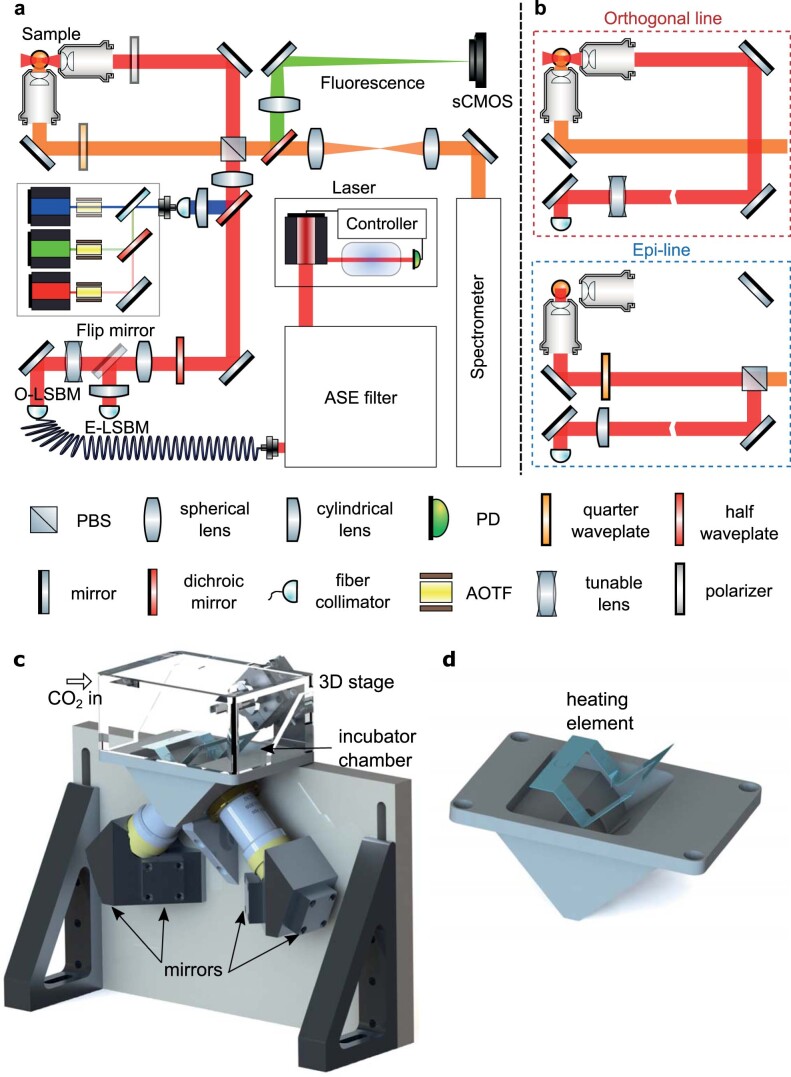
Extended Data Fig. 1
Optical and mechanical design of the LSBM.
(a) Conceptual schematic of the optical layout including both the fluorescence and Brillouin imaging modalities. The ASE filter and spectrometer are further detailed in Extended Data Figs. 2 and 3 , r...
Extended Data Fig. 2
Characterization and filtering of Amplified Spontaneous Emission (ASE).
(a) Optical layout of the double-pass ASE filter. To stabilize the Fabry-Perot (FP) based filter over a long time a feedback-loop is realized via a photodiode, custom-written Arduino software and piez...
Extended Data Fig. 3
Optical design of the LSBM spectrometer.
(a) Orthogonal views of the optical components in the LSBM spectrometer with relevant distances; top shows the plane determined by the illumination line and the optical axis of the detection objective...
Extended Data Fig. 4
Optical characterization and precision measurement of the LSBM spectrometer.
Orthogonal views of a 0.3um bead (Tetraspeck, Thermo Fischer) to characterize the optical resolution in the orthogonal (a) and epi line (b) geometries. (c) Spatial calibration (u00b5m to pixel) acquir...
Extended Data Fig. 5
Spectral characterization of the LSBM spectrometer.
(a) Acquired, raw spectra of the 4 hyperfine D2 spectral lines of Rb 85 and Rb 87 as measured by the LSBM spectrometer. (b) Frequency shift of the Rb lines in panel a after applying the reconstruction...
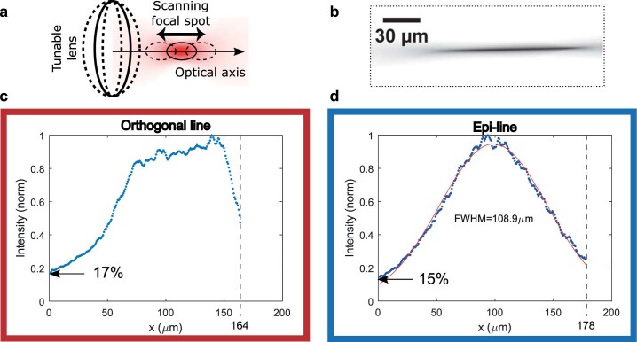
Extended Data Fig. 6
Characterization of the Brillouin illumination profile for both orthogonal and epi line geometries.
(a) Illustration of axial scanning by means of a tunable lens in order to extend the illumination depth and thus FOV in the orthogonal geometry. The curvature of the tunable lens can be controlled wit...
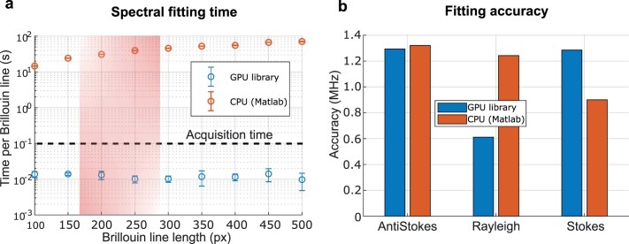
Extended Data Fig. 7
Performance of the GPU-accelerated spectral analysis pipeline.
(a) Brillouin spectrum fitting time as a function of image size (equal to number of independent spectra), comparing standard, CPU-based fitting routines (Matlab) and our custom GPU-accelerated library...
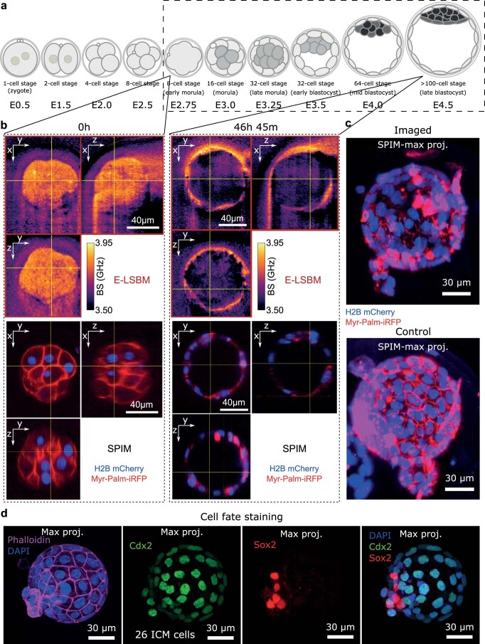
Extended Data Fig. 8
LSBM allows Brillouin time-lapse imaging of developing mouse embryos over ~2 days.
(a) Timeline of mouse embryo development from the one cell stage to late blastocyst. The dashed rectangle encloses the developmental window that was imaged. (b) Exemplary Brillouin volumes acquired in...
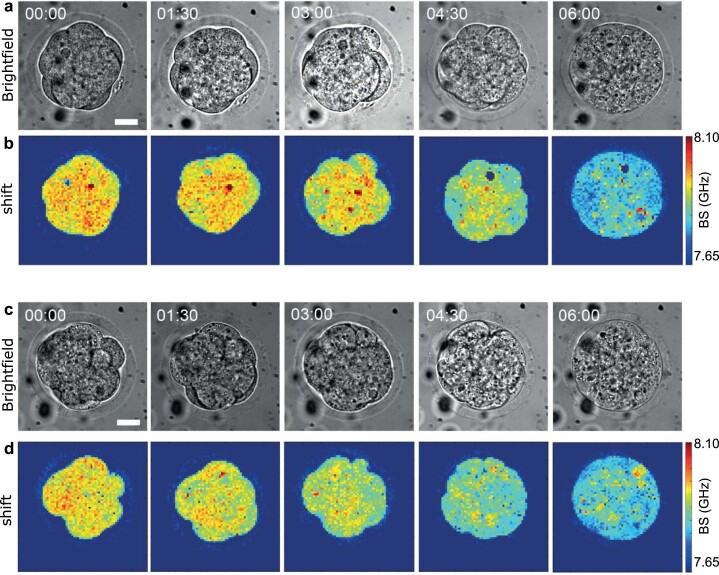
Extended Data Fig. 9
Embryos are not viable under 532-nm confocal Brillouin imaging.
(a) Bright-field images of an 8-cell stage mouse embryo that eventually undergoes cell death. ( b) Images of Brillouin shift for the same embryo as in a . ( c ) Another representative embryo (out of 3...
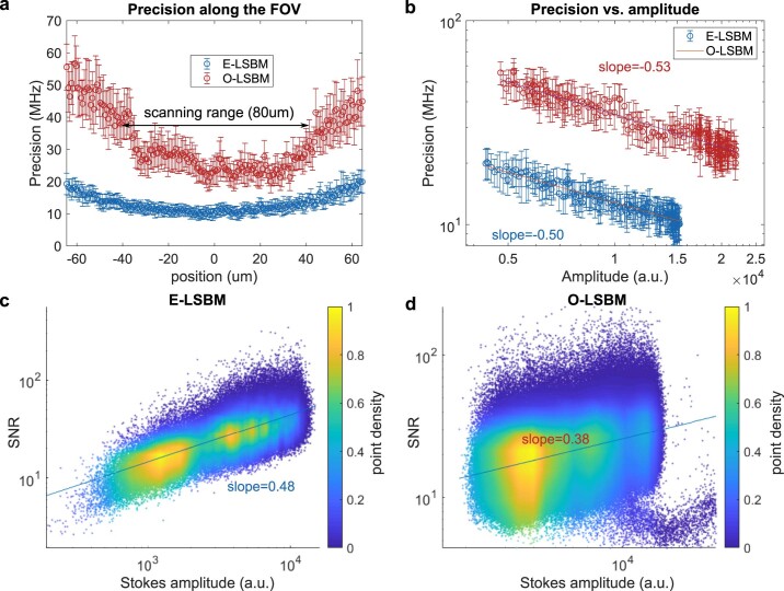
Extended Data Fig. 10
Performance characterization of LSBM.
(a) Analysis of the precision along the FOV for the O-LSBM (red) and E-LSBM (blue). (b) Analysis of the precision vs. amplitude along the FOV for the O-LSBM (red) and E-LSBM (blue). Data used for (a-b...
Figure images are served from the NIH/NLM PubMed Central Open Access Subset or Europe PMC; copyright remains with the publishers and authors.
💬 Discussion
0 commentsNo comments yet. Be the first to start a discussion!
Leave a Comment