Abstract
Episodic memory requires linking events in time, a function dependent on the hippocampus. In "trace" fear conditioning, animals learn to associate a neutral cue with an aversive stimulus despite their separation in time by a delay period on the order of tens of seconds. But how this temporal association forms remains unclear. Here we use two-photon calcium imaging of neural population dynamics throughout the course of learning and show that, in contrast to previous theories, hippocampal CA1 does not generate persistent activity to bridge the delay. Instead, learning is concomitant with broad changes in the active neural population. Although neural responses were stochastic in time, cue identity could be read out from population activity over longer timescales after learning. These results question the ubiquity of seconds-long neural sequences during temporal association learning and suggest that trace fear conditioning relies on mechanisms that differ from persistent activity accounts of working memory.
🔬 Techniques
✨ Fluorophores
🧪 Sample Preparation
🏭 Microscope Brands
🧪 Reagent Suppliers
📷 Detectors
🎨 Filters
💾 Data Repositories
🏛️ Research Organizations (ROR)
Affiliated research institutions:
📋 Methods
STAR*METHODS RESOURCE AVAILABILITY Lead Contact Further information and requests for resources and reagents should be directed to the Lead Contact, Attila Losonczy ( al2856@columbia.edu ).
Materials Availability
All unique resources generated in this study are available from the Lead Contact with a completed Materials Transfer Agreement.
Data and Code Availability
The data and analysis code generated in this study are available upon reasonable request to the corresponding authors.
EXPERIMENTAL MODEL AND SUBJECT DETAILS
All experiments were conducted in accordance with the NIH guidelines and with the approval of the Columbia University Institutional Animal Care and Use Committee. Experiments were performed with adult (8–16 weeks) male and female C57BL/6 mice (Jackson Laboratory) and transgenic CaMKIIα - Cre mice on a C57BL/6 background, where Cre is predominantly expressed in pyramidal neurons (R4Ag11 line, Dragatsis and Zeitlin (2000) ; Jackson Laboratory, Stock No: 027400). METHOD DETAILS Behavior and Imaging Viruses Optogenetic experiments were performed by bilaterally injecting (see below) either recombinant adeno-associated virus (rAAV) expressing ArchT (rAAV2/1- Syn-ArchT ) or tdTomato control protein (rAAV2/1- Syn-tdTom ), under the Synapsin promoter, into male and female C57BL/6 mice. These viruses were the generous gift of Dr. Boris Zemelman. Imaging experiments were performed by injecting Cre -dependent recombinant adeno-associated virus (rAAV) expressing GCaMP6f (rAAV1- Syn-Flex-GCaMP6f-WPRE-SV40 , Addgene/Penn Vector Core) into male and female transgenic CaMKIIα-Cre mice ( Dragatsis and Zeitlin, 2000 ) to label pyramidal neurons.
Show full methods section
STAR*METHODS RESOURCE AVAILABILITY Lead Contact Further information and requests for resources and reagents should be directed to the Lead Contact, Attila Losonczy ( al2856@columbia.edu ).
Materials Availability
All unique resources generated in this study are available from the Lead Contact with a completed Materials Transfer Agreement.
Data and Code Availability
The data and analysis code generated in this study are available upon reasonable request to the corresponding authors.
EXPERIMENTAL MODEL AND SUBJECT DETAILS
All experiments were conducted in accordance with the NIH guidelines and with the approval of the Columbia University Institutional Animal Care and Use Committee. Experiments were performed with adult (8–16 weeks) male and female C57BL/6 mice (Jackson Laboratory) and transgenic CaMKIIα - Cre mice on a C57BL/6 background, where Cre is predominantly expressed in pyramidal neurons (R4Ag11 line, Dragatsis and Zeitlin (2000) ; Jackson Laboratory, Stock No: 027400). METHOD DETAILS Behavior and Imaging Viruses Optogenetic experiments were performed by bilaterally injecting (see below) either recombinant adeno-associated virus (rAAV) expressing ArchT (rAAV2/1- Syn-ArchT ) or tdTomato control protein (rAAV2/1- Syn-tdTom ), under the Synapsin promoter, into male and female C57BL/6 mice. These viruses were the generous gift of Dr. Boris Zemelman. Imaging experiments were performed by injecting Cre -dependent recombinant adeno-associated virus (rAAV) expressing GCaMP6f (rAAV1- Syn-Flex-GCaMP6f-WPRE-SV40 , Addgene/Penn Vector Core) into male and female transgenic CaMKIIα-Cre mice ( Dragatsis and Zeitlin, 2000 ) to label pyramidal neurons.
Surgical procedure Viral delivery to hippocampal area
CA1 and implantation of headposts, optical fibers, and imaging cannulae were as described previously ( Kaifosh et al., 2013 ; Kheirbek et al., 2013 ; Lovett-Barron et al., 2014 ). Briefly, mice were anesthetized under isofluorane and viruses were delivered to dorsal CA1 by stereotactically injecting 50 nL (10 nL pulses) of rAAVs at three dorsoventral locations using a Nanoject syringe (−2.3 mm AP; −1.5 mm ML; −0.9, −1.05 and −1.2 mm DV relative to bregma). For head-fixed optogenetic experiments, mice were chronically implanted with bilateral optical fiber cannulae above the CA1 injection sites immediately after virus delivery ( Lovett-Barron et al., 2014 ; Kheirbek et al., 2013 ). A stainless steel headpost was then fixed to the skull ( Kaifosh et al., 2013 ). The cannula, headpost, and any exposed skull were secured and covered with black grip cement to block light from the implanted optical fibers. For imaging experiments, mice were allowed to recover in their home cage for 3 days following virus delivery procedures. They were then surgically implanted with a custom metal headpost (stainless steel or titanium) along with an imaging window (diameter, 3.0 mm; height, 1.5 mm or 2.3 mm) over the left dorsal hippocampus. Imaging cannulae were constructed by adhering (Narland optical adhesive) a 3 mm glass coverslip (64–0720, Warner) to a cylindrical steel cannula. The imaging window surgical procedure was performed as detailed previously ( Kaifosh et al., 2013 ; Lovett-Barron et al., 2014 ). Briefly, mice were anesthetized and the skull was exposed. A 3 mm hole was made in the skull over the virus injection site. Dura and cortical layers were gently removed under visual guidance while flushing with ice-cold cortex buffer. The imaging cannula was inserted through the surgical opening in the skull and secured so that external capsule fibers were visible through the cannula glass. Finally, the metal headpost was affixed to the skull with dental cement. For all surgeries, monitoring and analgesia (buprenorphine or meloxicam as needed) was continued for 3 days postoperatively. Behavioral apparatus We adopted our previously described ( Kaifosh et al., 2013 ; Lovett-Barron et al., 2014 ) head-fixed system for combining 2-photon imaging with microcontroller-driven (Arduino) stimulus presentation and behavioral readout. To maintain immobility and constrain neural activity related to locomotion ( MacDonald et al., 2013 ), mice were head-fixed in a body tube chamber ( Guo et al., 2014 ). The chamber was lined with textured fabric that was interchanged between trials to control for mouse excretions and prevent contextual conditioning. Tones were presented via nearby speakers and air-puffs delivered by actuating a solenoid valve, which gated airflow from a compressed air tank to a pipette tip pointed at the mouse’s snout. Water reward delivery during licking behavior was gated by another solenoid valve in response to tongue contact with a metal water port coupled to a capacitive sensor. Electrical signals encoding mouse behavior and stimulus presentation were collected with an analog-to-digital converter, which was synchronized with either optogenetic laser delivery or 2-photon image acquisition by a common trigger pulse. Head-fixed trace fear conditioning Starting 3–7 days after surgical implantation, mice were habituated to handling and head-fixation as previously described ( Kaifosh et al., 2013 ; Lovett-Barron et al., 2014 ; Guo et al., 2014 ). Within 3 days, mice could undergo up to an hour of head-fixation on the behavioral apparatus while remaining calm and alert. They were then water deprived to 85%–90% of their starting body weight and trained to lick operantly for small-volume water rewards (~500 nL/lick) while head-fixed. Before undergoing experimental paradigms, mice were required to maintain consistent licking for multiple (6–12) 60 s trials per day while maintaining their body weight between 85%–90% of starting weight. For optogenetic experiments, we utilized our previously described head-fixed ‘trace’ fear conditioning paradigm ( Kaifosh et al., 2013 ). Briefly, we paired a 20 s auditory conditioned stimulus (CS, either 10 kHz constant tone or 2 kHz tone pulsed at 1Hz) with air-puffs (unconditioned stimulus, US; 200 ms, 5 puffs at 1 Hz), separated by a 15 s stimulus-free ‘trace’ period. During each conditioning trial, we recorded licking from mice over a 50 s period: 10 s pre-CS, 20 s CS, 15 s trace, and 5 s US. Mice were conditioned across trials spaced throughout three consecutive days. On each trial, we used suppression of licking during the tone, normalized to licking during the 10 s pre-CS period, as a measure of conditioned fear. We changed the fabric material in the behavioral chamber between every trial to prevent contextual fear conditioning ( Kaifosh et al., 2013 ; Lovett-Barron et al., 2014 ). For 2-photon imaging experiments, we expanded our behavioral paradigm to a differential learning assay using the 2 different auditory cues above as either a CS+ or CS− (where only CS+ is paired with the aversive US). We randomized the assignment of CS+ and CS− tones across mice. Prior to the introduction of US-paired conditioning trials, we obtained multiple trials of behavioral responses (10–15 trials; “Pre-Learning”) to each CS cue presented alone in pseudorandom order over 2–3 days. Mice underwent blocks of 4–6 trials with 1–5 min inter-trial intervals each day (¿1 hour between trial blocks). We then subjected mice to our 3-day conditioning protocol with US-pairing as above, but with alternation between CS+ and CS− trials (“Learning”). Finally, over another 2–3 days, we collected additional trials beyond where behavioral responses plateaued (~20–25 of each CS presented in pseudo-random order, with trial blocks of 4–6 trials as above, “Post-Learning”) with continued US reinforcement on CS+ trials (to avoid extinction). During Pre-Learning and Post-Learning trials, contextual cues, consisting of the chamber fabric material and a background odor of either 70% ethanol or 2% acetic acid, were randomly changed across trials. Head-fixed optogenetics 200 μm core, 0.37 numerical aperture (NA) multimode optical fibers were constructed as previously detailed ( Kheirbek et al., 2013 ). A splitter patch cable (Thorlabs) was used to couple bilaterally implanted optical fibers to a 532 nm laser (50 mW, OptoEngine) for ArchT activation while mice were head-fixed. All cables/connections were shielded to prevent light leak from laser stimuli and matching-color ambient LED illumination was continuously provided in the behavioral apparatus so as to prevent the laser activation from serving as a visual cue. After the 10 s pre-CS period on each trace fear conditioning trial, 10 mW of laser light was continuously delivered through each optical fiber for the entire CS-trace-US sequence. Experimenters were blinded to subject viral injections. After data collection, mice were processed for histology and recovery of optical fibers. Subjects were excluded from the study if the implant entered the hippocampus, if viral infection was not complete in dorsal CA1, or if there were signs of damage to the optical fiber that could have compromised intracranial light delivery.
2-photon microscopy
For imaging experiments, mice were habituated to the imaging apparatus (e.g., microscope/objective, laser, sounds of resonant scanner and shutters) during the training period. All imaging was conducted using a 2-photon 8 kHz resonant scanner (Bruker) and 40× NIR water immersion objective (Nikon, 0.8 NA, 3.5mm working distance). Images were acquired as either single plane (n = 3 mice) or dual-plane (n = 3 mice) data. For dual-plane acquisitions, we coupled a piezoelectric crystal to the objective as described in Danielson et al. (2016) , allowing for rapid displacement of the imaging plane in the z dimension, which permitted simultaneous data collection from CA1 neurons in 2 different optical sections. To align the CA1 pyramidal layer with the horizontal two-photon imaging plane, we adjusted the angle of the mouse’s head using two goniometers (±10° range, Edmund Optics). For excitation, we used a 920 nm laser (50–100 mW at objective back aperture, Coherent). Green (GCaMP6f) fluorescence was collected through an emission cube filter set (HQ525/70 m-2p) to a GaAsP photomultiplier tube detector (Hamamatsu, 7422P-40). A custom dual stage preamp (1.4 × 10⁵ dB, Bruker) was used to amplify signals prior to digitization. All experiments were performed at 1–2× digital zoom, covering ~166–332 mm × 166–332 mm per imaging plane. Dual-plane images (512 × 512 pixels each) were separated by 20 μm in the optical axis and acquired at ~8 Hz given a 30ms settling time of the piezo z-device. Single-plane data (512 × 512 pixels each) was collected at 30 Hz in the absence of the piezo z-device.
QUANTIFICATION AND STATISTICAL ANALYSIS Image preprocessing
All imaging data were pre-processed using the SIMA software package ( Kaifosh et al., 2014 ). For dual-plane acquired data, motion correction was performed separately on individual trials using a modified 2D hidden Markov model ( Dombeck et al., 2007 ; Kaifosh et al., 2013 ) in which the model was re-initialized on each plane in order to account for the settling time of the piezo. For motion correction of single-plane acquired data, trials were registered (non-rigid registration) using the Suite2p software package ( Pachitariu et al., 2017 ). All recordings were visually assessed for residual motion. In cases where motion artifacts were not adequately corrected, the affected data were discarded from further analysis. We then used the Suite2p software package ( Pachitariu et al., 2017 ) to identify spatial masks corresponding to neural region of interest (ROIs) and extract associated fluorescence signal within these spatial footprints, correcting for neuropil contamination. Identified ROIs were curated post hoc using the Suite2p graphical interface to exclude non-somatic components. For each session, we detected only a subset of neurons that were physically present in the FOV. Once signals were extracted for all sessions, we registered ROIs across each session as follows. We first chose the session with the largest number of detected neurons as the reference session, and then computed an affine transform between the time-averaged FOV of all other sessions to the reference. Transforms were visually inspected to verify accuracy. Using these transforms, we processed each session serially to register ROIs to a common neural pool across sessions. For a given session (referred to now as the current session), the calculated FOV transform was applied to all ROI masks to map them to the reference session coordinates. We calculated a distance matrix (using Jaccard similarity) that quantified the spatial overlap between all pairs of reference and current session ROIs. We then applied the Hungarian algorithm ( Kuhn, 1955 ) to identify the optimal pairs of reference and current ROIs. All pairs with a Jaccard distance below 0.5 were automatically accepted as the same ROI. For the remaining unpaired current ROIs, pairs were manually curated via an IPython notebook, which allowed the user to select the appropriate reference ROI to pair or enter the current ROI as a new ROI (i.e., not in the reference pool). Any current ROIs whose centroids were more than 50 pixels away from an unpaired reference ROI were automatically entered as new ROIs, to accelerate the curation. Once all ROIs for the current session were processed (either paired with a reference ROI or labeled as new), the new ROIs were appended to the reference list. The remaining sessions were then processed serially in the same fashion, where the reference ROI list is augmented on each step to include additional ROIs that were not presented in any previously processed session. Once all sessions were processed, this process yielded a complete list of reference ROIs and their identity in each individual session. As a final step, the reference ROIs were warped back to the FOVs of each individual session via affine transform and ROIs that fell outside the boundaries of any session FOV were discarded, so that all analyzed neurons were physically in view for all sessions. Inbound reference ROIs that were not functionally detected in any individual session were assumed to be silent in that session for subsequent analysis.
Neural data analysis Event detection
All fluorescence traces were deconvolved to detect putative spike events, using the OASIS implementation of the fast non-negative deconvolution algorithm ( Friedrich et al., 2017 ). Following spike inferencing, we discarded any events whose energy was below 4 median absolute deviations of the raw trace. This avoided including small events within the range of the noise, which could artificially inflate activity rates and correlations between neurons. Given the dominant sparsity of activity, we then discretized each ROI trace to indicate whether an event was present in each frame. Trials for each experiment were collected over the span of several days. Consequently, we found that discretization was necessary to prevent variations in imaging system parameters from exerting undue influences on the analysis, as this could introduce arbitrary variance in the scale of calcium events across sessions. Decoding All classifiers in the main text were support vector machines (SVM) with a linear kernel, using the implementation in scikit-learn ( Pedregosa et al., 2011 ). For cross-validation, data were randomly divided into two non-overlapping groups of trials, used for training and testing the classifiers (75/25% split). This procedure was repeated 100 times for each classifier with random training/test subdivisions and reported as the average across cross-validation folds. Trials were balanced by subsampling the overrepresented class, and all decoding results were compared against a null distribution built by repeating the analyses on appropriately shuffled surrogate data, which controlled for the effects of finite sampling. This is particularly important for fear learning paradigms such as ours, where trial counts are very limited. Decoding elapsed time We designed a decoder to predict the elapsed time during each trial, in order to assess whether there were consistent temporal dynamics in the neural data during the experiment, such as sequences of time cells. To illustrate the idea behind this analysis (see Figure 2B schematic), we can summarize the activity of the network at each point in time as a point in a high dimensional neural state space, where the axes in this space corresponds to the activity rate of each neuron. The state of the network at each point in time during a trial traces out a path of points in neural state space. If the neural dynamics continually evolve in time (e.g., time cell sequences), then the neural state at one point in time (t) should be different from the states that occur at points further away in time ( t + Δ t ), reflecting the recruitment of different neurons at each point in the sequence. If these dynamics are reliable across many trials, we should be able to train a linear decoder to accurately classify whether data came from one time point or the other, by finding the hyperplane that maximally separates data from time t and t + Δ t in the neural state space. By extending this analysis to compare all possible pairs of time points (i.e., for all possible Dts), we can identify moments during the task that exhibit reliable temporal dynamics across trials ( Bakhurin et al., 2017 ; Cueva et al., 2019 ). Time decoding was done separately for CS+ and CS− trials, and for Pre- and Post-Learning trial blocks, to assess differences between cues and over learning. We analyzed data during both the tone and trace period, for a total of 35 s on each trial. We averaged each neuron’s activity in non-overlapping 2.5 s bins, so that each trial was described by a sequence of 14 population vectors of activity in time. Our time decoder uses a 1 versus 1 approach through an ensemble of linear classifiers. For each pair of time bins in the experiment, we train a separate classifier to distinguish between population vectors of activity that came from those two time bins. For comparing 14 time bins, this results in a set of 91 binary classifiers trained on all unique time comparisons ( Bakhurin et al., 2017 ; Cueva et al., 2019 ). We first evaluated the performance of the individual classifiers by testing their ability to correctly label time bins from held out test trials, where in this analysis each classifier is tested only on time bins from the trial times that it was trained to discriminate. This result is presented as a matrix in Figure 2C , and demonstrates the linear separability of any two points in time during the task. We then used the decoder to perform a multi-class time prediction analysis. Here each population vector in a held-out test trial is presented to all pairwise classifiers, which “vote” on what time bin the data came from (i.e., for each possible time bin, we tabulate the number of classifiers that decided the population activity came from that time). We take the decoded time to be the time bin with the plurality of votes, and repeat this procedure across all sample population vectors in each test trial to decode the passage of time. For all time decoding analyses, we compare the classification accuracy or prediction error to a null distribution, which we calculate by repeating these analyses on 1000 surrogate datasets, where for each trial independently, we randomly permute the order of the time bins. This destroys any consistent temporal information across trials, while preserving the average firing rates and correlations between neurons within each trial. We repeated the above analyses at a coarser time resolution (5 s, yielding a sequence of 7 population vectors in each trial), as well as repeated the analysis for both fine and coarse time resolutions using a nonlinear SVM (RBF kernel via scikit-learn, Pedregosa et al. [2011] ), all of which produced similar results to those reported in the main text (see Figure S2A ). Decoding stimulus identity from instantaneous firing rates We also used a population decoding approach to assess the times in the experiment during which there was significant information about the stimulus identity in the neural data. This analysis can be schematized similar to that above, where the different CS cues are associated with different network states that can be reliably segregated in state space by a hyperplane ( Figure 3A ). On each trial, we averaged the activity of each neuron in non-overlapping 1 s bins. We then trained a separate linear classifier on each time bin to predict whether the population vector came from a CS+ or CS− trial. Classifiers were cross-validated as above on held-out test data. We similarly compared the classification accuracy for trial information to a null distribution, where here we repeated the decoding analysis on 1000 surrogate datasets where the CS trial label was randomly shuffled. Decoding from average firing rates We similarly assessed our ability to decode stimulus identity from the average firing rates of the neurons within a set trial period on each trial. This procedure is identical to the one outlined above, and we used it to assess our ability to decode the CS identity during the Pre-CS (−10 to 0 s), CS (0 to 20 s), Trace (20 to 35 s), US (35 to 40 s), and Post-US (40 to 170 s) periods of the trial ( Figure 4B ), as well as during the CS and trace periods combined (0 to 35 s, Figure 4A ). We additionally assessed how decoders learned at one time period in the task generalize to activity observed in other time periods, by constructing a cross-time period decoding analysis. Here on each cross-validation fold, we trained different decoders to predict CS identity from the activity during each trial period separately. Then on the held-out test data, we tested each decoder not only on the activity from the time period on which it was trained, but on the activity of all other time periods as well (e.g., train on CS, test on trace). The result is a matrix of pairwise trial period comparisons, where the columns indicate the time period used for training the classifier and the row indicate the time period for testing. These comparisons are not necessarily symmetric (e.g., we find that CS period decoders can be used to predict the cue when tested on trace-period activity better than the reverse).
Selectivity index analysis
To assess CS-selectivity at the level of single neurons, we computed a selectivity index as: S I = f + − f − f + + f − where f + and f − are the average activity of the neuron in the examined trial time period on CS+ and CS− trials, respectively. This yields an index bounded between +1 (all activity during CS+ trials) and −1 (all activity during CS trial). Similar to the decoding analysis, we compared this selectivity index to those calculated from 1000 surrogate datasets where the trial type labels were randomly shuffled, which controlled for spurious firing rate differences attributable to small numbers of trials. We computed these scores separately for Pre- and Post-Learning trials, and quantified the fraction of cells active during that trial type which showed significant CS-selectivity, determined by calculating a p value from the observed SI relative to its shuffle distribution. For the regression to population decoder weights shown in Figure 4E , we z-scored each SI (computed from average activity over CS and trace periods; 0–35 s) relative to its shuffle distribution’s mean and standard deviation. Sequence score For analysis of neural sequences using cell firing orders, we detected the latency to peak firing rate for each neuron during the CS and trace periods (0 to 35 s) that was active on at least one trial. We compared this firing order between all trial pairs via Spearman’s rank correlation, and assigned a sequence score as the average pairwise rank correlation between trials. This analysis was done separately for CS+ and CS− trials. To assess significance, sequence scores were compared to those calculated from 1000 surrogate datasets, where for each neuron, its activity trace was randomly permuted on each trial independently to randomize the temporal ordering between cells’ activity events.
Hidden Markov model
We used hidden Markov models (HMMs) as an additional, more flexible probe for sequential dynamics in the neural data ( Mazzucato et al., 2019 ; Maboudi et al., 2018 ). The HMM identifies a set of latent neural states, which can be thought of as a recurring pattern of population activity: each state dictates a probability for each neuron that it will be active when the network is in that state. The HMM is simultaneously a clustering algorithm which identifies periods of similar neural activity, and a model of neural sequences, as it models the transitions between latent states over time. We use this framework to analyze both the temporal and covariance structure of neural population activity. Formally, we model the neural states as evolving in time under first order Markovian dynamics. Let q denote the discrete state variable and { S 1 … S K } be the set of possible states. Then the probability of transitioning from one state q ( t ) = S i to the next q ( t + 1) = S j depends only on the current state, and these “transition” probabilities are described by a K × K matrix A with elements a ij : P ( q ( t + 1 ) = S j ) = P ( q ( t + 1 ) = S j | q ( t ) = S i ) = a i j The state variable q is never observed directly, but rather exerts an influence on the observed neural activity. Since we are working with binarized calcium events, it is natural to describe each neuron as an independent Bernoulli process, whose activation probability depends on the current neural state. Letting n i ( t ) be the activation of the i th neuron at time t which can take values ∈˛{0,1}, and { n 1 ( t )… n N ( t )} = n (t): P ( n i ( t ) | q ( t ) = s j ) ∼ Bernoulli [ b i j ] P ( n ( t ) | q ( t ) = s j ) = ∏ i = 1 N b i j n i ( t ) ( 1 − b i j ) 1 − n i ( t ) Here the b ij are elements of the “observation” matrix B , which summarizes the firing rates (activation probability) of the i th neuron when the network is in the j th state. In sum, the columns of B give us the pattern of activity observed when the network is in each neural state, and A describes how the network moves dynamically between states over time. Together with the vector π which describes the probability of starting in each state, the model is completely specified by these parameters { A,B, π} ( Rabiner, 1989 ). The HMM parameters { A,B ,π} are not known a priori and must be fit to the observed neural data. We used the standard Baum-Welch expectation-maximization algorithm to iteratively update the model parameters in order to maximize the likelihood of the data ( Rabiner, 1989 ), treating each trial as an observation sequence. During each M-step of the procedure, we enforced a minimum activity rate of 0.001 Hz to regularize the model ( Maboudi et al., 2018 ). The optimization is non-convex and prone to local minima, which we combated by first initializing B using a modified K -means clustering of the neural data. The hyperparameter K , which specifies the number of latent neural states in the model, is not learned and must be set manually. We fit 12 models to the dataset for each value of K ∈ {5…50}, using randomized initial conditions, and for each K we retained the model that maximized the likelihood of the data. We trained a separate set of models for Pre-Learning and Post-Learning trials, for each mouse.
HMM transition analysis
After fitting the model, we estimated the most likely sequence of states on each trial via the Viterbi algorithm ( Rabiner, 1989 ). From this sequence, we constructed single trial transition matrices by counting state transitions along the Viterbi path. Similar to the rank sequence analysis described previously, we computed the correlation between these transition matrices for all pairs of trials, as a measure of the similarity of trial activity sequences. For this calculation, we set the diagonal of each transition matrix to zero, so that the correlations focused on which state transitions appeared on a given trial, rather than the state duration implicit in self-transition probabilities. To determine significance, we compared this averaged sequence correlation to a distribution of correlations generated by randomly shuffling the order of time bins independently on each trial prior to calculation ( Recanatesi et al., 2020 ). This procedure was repeated for all model complexities, separately for CS+ and CS− trials. Decoding CS using HMM states For each trial, we calculated the posterior probability of each state at each point in time, given the model parameters and the observed neural data. From this, we estimated the frequency that each state appeared in the trial as the average of the state posterior probability over time ( Rabiner, 1989 ). Similar to our decoding analysis using mean firing rates described previously, we trained a linear SVM to decode the identity of the CS cue using the state frequencies on each trial, calculated from 0–35 s relative to the cue onset (i.e., CS and trace period). We gauged how much each state reflected strongly co-active neurons by counting the number of neurons whose observation probabilities exceeded 75%. We also assigned each state a CS selectivity ranking based on the absolute value of its weight in the decoder trained on state frequencies. We then plotted the average number of strongly co-active neurons in each state, separately for each selectivity rank ( Figure S3 ).
Ensemble overlap analysis
We measured the similarity in the active set of neurons between a pair of trials by computing the Jaccard similarity index, which for two sets is given by the size of the set intersection divided by the size of the set union ( Figure S4 ). Intuitively, if the sets of active neurons overlap completely, the set intersection and union are equal and the index is 1, while if trials recruit orthogonal sets of neurons, the intersection and thus the index are 0. This metric is biased by the fraction of active neurons on a given trial; if two trials randomly recruit 50% of neurons, the Jaccard similarity will tend to be higher than if they randomly recruited 10% of neurons, as the former will tend to have more overlapping elements purely by chance. To control for differences in activity rates across trials, we generated 1000 surrogate scores for each trial pair where we recomputed the index between two binary vectors whose elements were randomly assigned as active or inactive to match the fraction of active neurons in the real trials. The observed index was then z-normalized relative to this distribution, to quantify the population similarity beyond that expected from random recruitment of the same number of neurons.
Statistics
Statistical details of experiments can be found in the figure legends. Statistical details of analysis methods are described in the corresponding sections above. No statistical methods were used to predetermine sample sizes, but our sample sizes are similar to those reported in previous publications.
Materials Availability
All unique resources generated in this study are available from the Lead Contact with a completed Materials Transfer Agreement.
EXPERIMENTAL MODEL AND SUBJECT DETAILS
All experiments were conducted in accordance with the NIH guidelines and with the approval of the Columbia University Institutional Animal Care and Use Committee. Experiments were performed with adult (8–16 weeks) male and female C57BL/6 mice (Jackson Laboratory) and transgenic CaMKIIα - Cre mice on a C57BL/6 background, where Cre is predominantly expressed in pyramidal neurons (R4Ag11 line, Dragatsis and Zeitlin (2000) ; Jackson Laboratory, Stock No: 027400).
METHOD DETAILS Behavior and Imaging Viruses Optogenetic experiments were performed by bilaterally injecting (see below) either recombinant adeno-associated virus (rAAV) expressing ArchT (rAAV2/1- Syn-ArchT ) or tdTomato control protein (rAAV2/1- Syn-tdTom ), under the Synapsin promoter, into male and female C57BL/6 mice. These viruses were the generous gift of Dr. Boris Zemelman. Imaging experiments were performed by injecting Cre -dependent recombinant adeno-associated virus (rAAV) expressing GCaMP6f (rAAV1- Syn-Flex-GCaMP6f-WPRE-SV40 , Addgene/Penn Vector Core) into male and female transgenic CaMKIIα-Cre mice ( Dragatsis and Zeitlin, 2000 ) to label pyramidal neurons.
Surgical procedure Viral delivery to hippocampal area
CA1 and implantation of headposts, optical fibers, and imaging cannulae were as described previously ( Kaifosh et al., 2013 ; Kheirbek et al., 2013 ; Lovett-Barron et al., 2014 ). Briefly, mice were anesthetized under isofluorane and viruses were delivered to dorsal CA1 by stereotactically injecting 50 nL (10 nL pulses) of rAAVs at three dorsoventral locations using a Nanoject syringe (−2.3 mm AP; −1.5 mm ML; −0.9, −1.05 and −1.2 mm DV relative to bregma). For head-fixed optogenetic experiments, mice were chronically implanted with bilateral optical fiber cannulae above the CA1 injection sites immediately after virus delivery ( Lovett-Barron et al., 2014 ; Kheirbek et al., 2013 ). A stainless steel headpost was then fixed to the skull ( Kaifosh et al., 2013 ). The cannula, headpost, and any exposed skull were secured and covered with black grip cement to block light from the implanted optical fibers. For imaging experiments, mice were allowed to recover in their home cage for 3 days following virus delivery procedures. They were then surgically implanted with a custom metal headpost (stainless steel or titanium) along with an imaging window (diameter, 3.0 mm; height, 1.5 mm or 2.3 mm) over the left dorsal hippocampus. Imaging cannulae were constructed by adhering (Narland optical adhesive) a 3 mm glass coverslip (64–0720, Warner) to a cylindrical steel cannula. The imaging window surgical procedure was performed as detailed previously ( Kaifosh et al., 2013 ; Lovett-Barron et al., 2014 ). Briefly, mice were anesthetized and the skull was exposed. A 3 mm hole was made in the skull over the virus injection site. Dura and cortical layers were gently removed under visual guidance while flushing with ice-cold cortex buffer. The imaging cannula was inserted through the surgical opening in the skull and secured so that external capsule fibers were visible through the cannula glass. Finally, the metal headpost was affixed to the skull with dental cement. For all surgeries, monitoring and analgesia (buprenorphine or meloxicam as needed) was continued for 3 days postoperatively. Behavioral apparatus We adopted our previously described ( Kaifosh et al., 2013 ; Lovett-Barron et al., 2014 ) head-fixed system for combining 2-photon imaging with microcontroller-driven (Arduino) stimulus presentation and behavioral readout. To maintain immobility and constrain neural activity related to locomotion ( MacDonald et al., 2013 ), mice were head-fixed in a body tube chamber ( Guo et al., 2014 ). The chamber was lined with textured fabric that was interchanged between trials to control for mouse excretions and prevent contextual conditioning. Tones were presented via nearby speakers and air-puffs delivered by actuating a solenoid valve, which gated airflow from a compressed air tank to a pipette tip pointed at the mouse’s snout. Water reward delivery during licking behavior was gated by another solenoid valve in response to tongue contact with a metal water port coupled to a capacitive sensor. Electrical signals encoding mouse behavior and stimulus presentation were collected with an analog-to-digital converter, which was synchronized with either optogenetic laser delivery or 2-photon image acquisition by a common trigger pulse. Head-fixed trace fear conditioning Starting 3–7 days after surgical implantation, mice were habituated to handling and head-fixation as previously described ( Kaifosh et al., 2013 ; Lovett-Barron et al., 2014 ; Guo et al., 2014 ). Within 3 days, mice could undergo up to an hour of head-fixation on the behavioral apparatus while remaining calm and alert. They were then water deprived to 85%–90% of their starting body weight and trained to lick operantly for small-volume water rewards (~500 nL/lick) while head-fixed. Before undergoing experimental paradigms, mice were required to maintain consistent licking for multiple (6–12) 60 s trials per day while maintaining their body weight between 85%–90% of starting weight. For optogenetic experiments, we utilized our previously described head-fixed ‘trace’ fear conditioning paradigm ( Kaifosh et al., 2013 ). Briefly, we paired a 20 s auditory conditioned stimulus (CS, either 10 kHz constant tone or 2 kHz tone pulsed at 1Hz) with air-puffs (unconditioned stimulus, US; 200 ms, 5 puffs at 1 Hz), separated by a 15 s stimulus-free ‘trace’ period. During each conditioning trial, we recorded licking from mice over a 50 s period: 10 s pre-CS, 20 s CS, 15 s trace, and 5 s US. Mice were conditioned across trials spaced throughout three consecutive days. On each trial, we used suppression of licking during the tone, normalized to licking during the 10 s pre-CS period, as a measure of conditioned fear. We changed the fabric material in the behavioral chamber between every trial to prevent contextual fear conditioning ( Kaifosh et al., 2013 ; Lovett-Barron et al., 2014 ). For 2-photon imaging experiments, we expanded our behavioral paradigm to a differential learning assay using the 2 different auditory cues above as either a CS+ or CS− (where only CS+ is paired with the aversive US). We randomized the assignment of CS+ and CS− tones across mice. Prior to the introduction of US-paired conditioning trials, we obtained multiple trials of behavioral responses (10–15 trials; “Pre-Learning”) to each CS cue presented alone in pseudorandom order over 2–3 days. Mice underwent blocks of 4–6 trials with 1–5 min inter-trial intervals each day (¿1 hour between trial blocks). We then subjected mice to our 3-day conditioning protocol with US-pairing as above, but with alternation between CS+ and CS− trials (“Learning”). Finally, over another 2–3 days, we collected additional trials beyond where behavioral responses plateaued (~20–25 of each CS presented in pseudo-random order, with trial blocks of 4–6 trials as above, “Post-Learning”) with continued US reinforcement on CS+ trials (to avoid extinction). During Pre-Learning and Post-Learning trials, contextual cues, consisting of the chamber fabric material and a background odor of either 70% ethanol or 2% acetic acid, were randomly changed across trials. Head-fixed optogenetics 200 μm core, 0.37 numerical aperture (NA) multimode optical fibers were constructed as previously detailed ( Kheirbek et al., 2013 ). A splitter patch cable (Thorlabs) was used to couple bilaterally implanted optical fibers to a 532 nm laser (50 mW, OptoEngine) for ArchT activation while mice were head-fixed. All cables/connections were shielded to prevent light leak from laser stimuli and matching-color ambient LED illumination was continuously provided in the behavioral apparatus so as to prevent the laser activation from serving as a visual cue. After the 10 s pre-CS period on each trace fear conditioning trial, 10 mW of laser light was continuously delivered through each optical fiber for the entire CS-trace-US sequence. Experimenters were blinded to subject viral injections. After data collection, mice were processed for histology and recovery of optical fibers. Subjects were excluded from the study if the implant entered the hippocampus, if viral infection was not complete in dorsal CA1, or if there were signs of damage to the optical fiber that could have compromised intracranial light delivery.
2-photon microscopy
For imaging experiments, mice were habituated to the imaging apparatus (e.g., microscope/objective, laser, sounds of resonant scanner and shutters) during the training period. All imaging was conducted using a 2-photon 8 kHz resonant scanner (Bruker) and 40× NIR water immersion objective (Nikon, 0.8 NA, 3.5mm working distance). Images were acquired as either single plane (n = 3 mice) or dual-plane (n = 3 mice) data. For dual-plane acquisitions, we coupled a piezoelectric crystal to the objective as described in Danielson et al. (2016) , allowing for rapid displacement of the imaging plane in the z dimension, which permitted simultaneous data collection from CA1 neurons in 2 different optical sections. To align the CA1 pyramidal layer with the horizontal two-photon imaging plane, we adjusted the angle of the mouse’s head using two goniometers (±10° range, Edmund Optics). For excitation, we used a 920 nm laser (50–100 mW at objective back aperture, Coherent). Green (GCaMP6f) fluorescence was collected through an emission cube filter set (HQ525/70 m-2p) to a GaAsP photomultiplier tube detector (Hamamatsu, 7422P-40). A custom dual stage preamp (1.4 × 10⁵ dB, Bruker) was used to amplify signals prior to digitization. All experiments were performed at 1–2× digital zoom, covering ~166–332 mm × 166–332 mm per imaging plane. Dual-plane images (512 × 512 pixels each) were separated by 20 μm in the optical axis and acquired at ~8 Hz given a 30ms settling time of the piezo z-device. Single-plane data (512 × 512 pixels each) was collected at 30 Hz in the absence of the piezo z-device.
Surgical procedure Viral delivery to hippocampal area
CA1 and implantation of headposts, optical fibers, and imaging cannulae were as described previously ( Kaifosh et al., 2013 ; Kheirbek et al., 2013 ; Lovett-Barron et al., 2014 ). Briefly, mice were anesthetized under isofluorane and viruses were delivered to dorsal CA1 by stereotactically injecting 50 nL (10 nL pulses) of rAAVs at three dorsoventral locations using a Nanoject syringe (−2.3 mm AP; −1.5 mm ML; −0.9, −1.05 and −1.2 mm DV relative to bregma). For head-fixed optogenetic experiments, mice were chronically implanted with bilateral optical fiber cannulae above the CA1 injection sites immediately after virus delivery ( Lovett-Barron et al., 2014 ; Kheirbek et al., 2013 ). A stainless steel headpost was then fixed to the skull ( Kaifosh et al., 2013 ). The cannula, headpost, and any exposed skull were secured and covered with black grip cement to block light from the implanted optical fibers. For imaging experiments, mice were allowed to recover in their home cage for 3 days following virus delivery procedures. They were then surgically implanted with a custom metal headpost (stainless steel or titanium) along with an imaging window (diameter, 3.0 mm; height, 1.5 mm or 2.3 mm) over the left dorsal hippocampus. Imaging cannulae were constructed by adhering (Narland optical adhesive) a 3 mm glass coverslip (64–0720, Warner) to a cylindrical steel cannula. The imaging window surgical procedure was performed as detailed previously ( Kaifosh et al., 2013 ; Lovett-Barron et al., 2014 ). Briefly, mice were anesthetized and the skull was exposed. A 3 mm hole was made in the skull over the virus injection site. Dura and cortical layers were gently removed under visual guidance while flushing with ice-cold cortex buffer. The imaging cannula was inserted through the surgical opening in the skull and secured so that external capsule fibers were visible through the cannula glass. Finally, the metal headpost was affixed to the skull with dental cement. For all surgeries, monitoring and analgesia (buprenorphine or meloxicam as needed) was continued for 3 days postoperatively.
📊 Figures
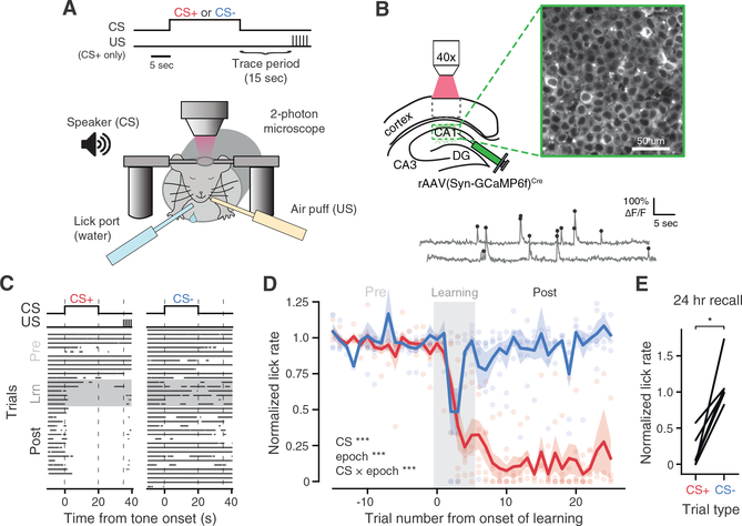
Figure 1.
Two-Photon Functional Imaging of CA1 Pyramidal Neurons during Differential tFC
(A) Schematic of experimental paradigm. A head-fixed mouse is immobilized and on each trial exposed to an auditory cue (CS+ or CSu2212) for 20 s, followed by a 15 s stimulus-free u201ctraceu201d perio...
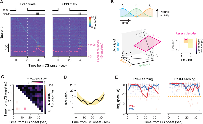
Figure 2.
Temporal Dynamics of CA1 Activity during tFC
(A) Summary of neural activity during Post-Learning CS+ trials, shown separately for even- and odd-numbered trials. Activity is trial averaged and sorted byneuronsu2019 peak firing rate latency during...
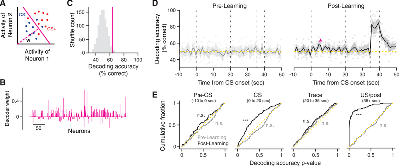
Figure 3.
CS Identity Is Not Persistently Encoded in the Moment-to-Moment Activity of CA1
(A) Schematic of CS decoding analysis. A separate classifier was trained to discriminate between CS+ and CSu2212 trials using population activity at each time point during the task (1 s bins). (B) Neu...
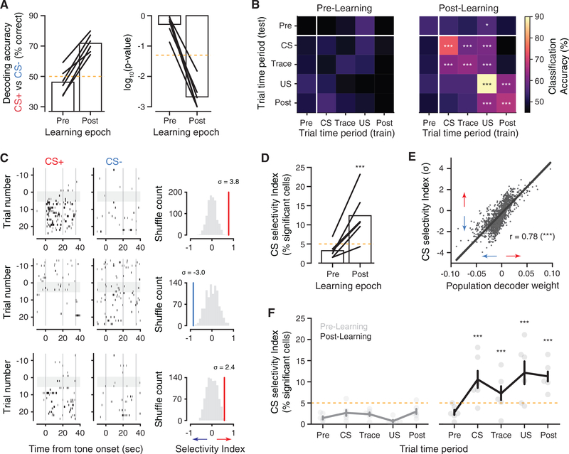
Figure 4.
CS Identity Is Predicted by CA1 Activity Rates on Longer Timescales
(A) CS decoding accuracy for classifiers trained on the average activity within each trialu2019s CS and trace period. Left: percentage accuracy; right: p value from nulldistributions calculated as in ...
Figure images are served from the NIH/NLM PubMed Central Open Access Subset or Europe PMC; copyright remains with the publishers and authors.
💬 Discussion
0 commentsNo comments yet. Be the first to start a discussion!
Leave a Comment