Abstract
AbstractTo study the development and interactions of cells and tissues, multiple fluorescent markers need to be imaged efficiently in a single living organism. Instead of acquiring individual colours sequentially with filters, we created a platform based on line-scanning light sheet microscopy to record the entire spectrum for each pixel in a three-dimensional volume. We evaluated data sets with varying spectral sampling and determined the optimal channel width to be around 5 nm. With the help of these data sets, we show that our setup outperforms filter-based approaches with regard to image quality and discrimination of fluorophores. By spectral unmixing we resolved overlapping fluorophores with up to nanometre resolution and removed autofluorescence in zebrafish and fruit fly embryos.
🔬 Techniques
🧬 Organisms
💻 Software
✨ Fluorophores
🏭 Microscope Brands
🧪 Reagent Suppliers
📷 Detectors
💻 Software Details
🏛️ Research Organizations (ROR)
Affiliated research institutions:
📋 Methods
Setup
A schematic of the hyperspectral SPIM setup can be found in Supplementary Fig. 2 and the optical properties of the components are listed in Supplementary Table 1 . The hyperspectral SPIM consisted of two identical water-dipping Nikon CLI75 16x/0.8 objectives that were inserted into the custom-made acrylic sample chamber through openings sealed with O-rings. One objective was used for illumination, one for detection. The sample was inserted from the top and moved with an xyz manual translation stage (M-460A-XYZ, Newport, USA) to ensure correct positioning at the intersection of the focal planes of illumination and detection objective. For stack acquisition, the sample was moved in z -direction with a motorized linear stage (M111.1DG, Physik Instrumente, Germany). An LED (CCS TH-27/27-SW, Stemmer imaging GmbH, Germany) was placed opposite of the detection objective for bright field illumination. For light sheet illumination, a multicolour laser light engine (SOLE-6, Omicron-Laserage Laserprodukte GmbH, Germany) with 405 nm (120 mW), 488 nm (200 mW) and 561 nm (150 mW) lasers was used. While scattered laser light could also be removed computationally by discarding the affected wavelengths from the hyperspectral data sets, bright signal might bleed into neighbouring pixels and was therefore suppressed with filters. Depending on the illumination scheme (single wavelength versus multiple wavelengths), scattered laser light was blocked with a 488 LP Edge Basic Filter (Chroma Technology Corporation, USA) or a Quad-Notch Filter 400–410/488/561/631–640 (Semrock, USA). Since several fluorophores could be excited with a single wavelength (for example, GFP and YFP), our illumination scheme with three excitation wavelengths and a Quad-Notch Filter was sufficient for many available fluorophores. A list of laser lines, filters and fluorescent markers used for each presented acquisition can be found in Supplementary Table 2 . In both the detection and illumination arms, a 4 f -system of tube and scan lens was used to image the objective lenses' back focal plane onto the scan and descan mirrors (dynAXIS M, Scanlab AG, Germany). The mirrors were driven with an analogue output card (NI PCI-6733, National Instruments Corporation, USA). In the illumination arm, the scan mirror was used to form the light sheet, whereas the descanning mirror in the detection arm projected the fluorescence from the illuminated part of the sample onto a single line. An imaging spectrograph was placed with its entrance slit in the image plane of this line, separating the incoming multicolour signal spatially. Depending on the spectral sampling and acquisition time required, we used either the Imspector V8E (Specim, Finland) for slow acquisitions with a spectral sampling of 0.5 nm per pixel or an Imspector FAST10 for high acquisition speeds with a reduced spectral sampling of 5 nm per pixel. The x, λ -image formed by the imaging spectrograph was recorded with an sCMOS camera (Zyla 5.5, Andor, United Kingdom), which was attached to the C-mount of the imaging spectrograph. The overall magnification of the system was determined to be 13.75. A 45° flip mirror was placed behind the tube lens and a CCD camera (Stingray F-145 B/C, Allied Vision Tech, USA) was used to observe a DSLM-like wide-field image and to facilitate sample positioning. Before measurements, the field of view on the Stingray was checked to match the field of view of the Imspector-Zyla assembly with a bead sample.
Show full methods section
Setup
A schematic of the hyperspectral SPIM setup can be found in Supplementary Fig. 2 and the optical properties of the components are listed in Supplementary Table 1 . The hyperspectral SPIM consisted of two identical water-dipping Nikon CLI75 16x/0.8 objectives that were inserted into the custom-made acrylic sample chamber through openings sealed with O-rings. One objective was used for illumination, one for detection. The sample was inserted from the top and moved with an xyz manual translation stage (M-460A-XYZ, Newport, USA) to ensure correct positioning at the intersection of the focal planes of illumination and detection objective. For stack acquisition, the sample was moved in z -direction with a motorized linear stage (M111.1DG, Physik Instrumente, Germany). An LED (CCS TH-27/27-SW, Stemmer imaging GmbH, Germany) was placed opposite of the detection objective for bright field illumination. For light sheet illumination, a multicolour laser light engine (SOLE-6, Omicron-Laserage Laserprodukte GmbH, Germany) with 405 nm (120 mW), 488 nm (200 mW) and 561 nm (150 mW) lasers was used. While scattered laser light could also be removed computationally by discarding the affected wavelengths from the hyperspectral data sets, bright signal might bleed into neighbouring pixels and was therefore suppressed with filters. Depending on the illumination scheme (single wavelength versus multiple wavelengths), scattered laser light was blocked with a 488 LP Edge Basic Filter (Chroma Technology Corporation, USA) or a Quad-Notch Filter 400–410/488/561/631–640 (Semrock, USA). Since several fluorophores could be excited with a single wavelength (for example, GFP and YFP), our illumination scheme with three excitation wavelengths and a Quad-Notch Filter was sufficient for many available fluorophores. A list of laser lines, filters and fluorescent markers used for each presented acquisition can be found in Supplementary Table 2 . In both the detection and illumination arms, a 4 f -system of tube and scan lens was used to image the objective lenses' back focal plane onto the scan and descan mirrors (dynAXIS M, Scanlab AG, Germany). The mirrors were driven with an analogue output card (NI PCI-6733, National Instruments Corporation, USA). In the illumination arm, the scan mirror was used to form the light sheet, whereas the descanning mirror in the detection arm projected the fluorescence from the illuminated part of the sample onto a single line. An imaging spectrograph was placed with its entrance slit in the image plane of this line, separating the incoming multicolour signal spatially. Depending on the spectral sampling and acquisition time required, we used either the Imspector V8E (Specim, Finland) for slow acquisitions with a spectral sampling of 0.5 nm per pixel or an Imspector FAST10 for high acquisition speeds with a reduced spectral sampling of 5 nm per pixel. The x, λ -image formed by the imaging spectrograph was recorded with an sCMOS camera (Zyla 5.5, Andor, United Kingdom), which was attached to the C-mount of the imaging spectrograph. The overall magnification of the system was determined to be 13.75. A 45° flip mirror was placed behind the tube lens and a CCD camera (Stingray F-145 B/C, Allied Vision Tech, USA) was used to observe a DSLM-like wide-field image and to facilitate sample positioning. Before measurements, the field of view on the Stingray was checked to match the field of view of the Imspector-Zyla assembly with a bead sample.
Wavelength calibration
In order to calibrate the recorded wavelengths, the spectrum of each laser line of the SOLE-6 (405, 488, 514, 561, 594 and 638 nm) was recorded once with a spectrometer (USB4000 Miniature Fiber Optic Spectrometer, Ocean Optics, USA). On each day of measurements, all filters were removed and the scattered signal of all six laser lines was recorded simultaneously on the camera chip. The intensities of both measurements were fitted with Gaussian distributions to determine the centre positions using a MATLAB (MathWorks, USA) script. The acquired centre positions were fitted linearly to obtain the calibration curve ( Supplementary Fig. 3 ). This calibration is fast and can be easily repeated on each day of measurements to ensure precise and reproducible spectra.
Acquisition and online reconstruction of descanned data
During data acquisition, lasers, scan mirrors and motorized stage were controlled via a LabVIEW (National Instruments) interface. To ensure precise synchronization, the camera received a digital trigger when the scan and descan mirrors began moving synchronously to scan the laser through the sample and descan onto the camera, respectively ( Supplementary Fig. 5 ). Laser powers for imaging were set between 2 and 10 mW in the back focal plane of the illumination objective, depending on laser colour and brightness of the fluorescent marker. For the Imspector VE8, the camera typically acquired a stack consisting of around 2,000 x , λ -images of 2,000 × 660 pixel (spatial × spectral). With a dynamic range of 16 bit, this amounts to 5 GB of data per acquired z -plane. The camera was run at 285 fps, which was the maximum possible frame rate for the chosen image size, amounting to a total acquisition time of 7 s for the whole λ -stack. For the Imspector FAST10, only 70 spectral channels were acquired. Therefore, a typical stack consisted of 2,000 x , λ -images of 2,000 × 70 pixel, amounting to 500 MB per z -plane. For this stack size, the camera was run at almost 1,500 fps, reducing the acquisition time to 1.5 s. A Fiji 18 plugin using the Java Native Interface for function calls into the Andor Software Development Kit was used to control camera settings and read the images from the camera. The same plugin transformed the acquired y -stacks into λ -stacks in real time.
Linear unmixing and data visualization
In order to separate the acquired spectral data according to the contributions of the individual dyes, a Fiji plugin implementing a blind linear unmixing algorithm 17 was adapted to our data sets. In brief, the algorithm adjusted both the spectra and concentrations for each dye in each pixel iteratively. The update rules were designed to assume a Poissonian distribution of photon counts. When unmixing was completed, a multichannel image and the spectra of each contributing dye were obtained. Fiji was used to visualize the acquired λ -stacks and unmixed images. To visualize the obtained spectra, LibreOffice (The Document Foundation) was used. Literature values for the spectra were obtained from the collection on the Tsien-lab homepage 16 .
Optimal spectral sampling for hyperspectral imaging
In our line-scanning hyperspectral SPIM, acquisition time increased linearly with spectral sampling. Furthermore, high spectral sampling might have adverse effects on image quality, since spreading of the fluorescence signal across many camera lines was expected to reduce SNR. On the other hand, it may no longer be possible to discriminate between different fluorophores with reduced spectral sampling. We determined the optimal spectral sampling for hyperspectral imaging by calculating image quality and the ability to discriminate different fluorophores (avoiding bleedthrough, BT). We defined the SNR of the whole image area as a measure for image quality in each channel where the pixels containing signal were selected by mean thresholding and the background was determined from an image area not containing any relevant signal; x FP denotes fluorescent protein x and y FP fluorescent protein y . As a measure for BT into each channel, we calculated the SNR of regions containing only one fluorophore, SNR x FP, y FP and determined their ratios where the subscript x FP denotes ‘expected' signal (i. e. GFP signal in the GFP channel) and the subscript y FP ‘unexpected' signal (YFP signal in the GFP channel). Overall SNR and BT were determined as root mean square of the values from each channel In order to determine the optimal regime, we created a 200 × 200 pixel synthetic data set containing three spots with a Gaussian intensity distribution in MATLAB. One of these spots was multiplied with a GFP spectrum obtained from measurements, one with a YFP spectrum and the third with the mean of both spectra. From this simulated data set with a spectral sampling of 0.5 nm per pixel, we generated data with reduced spectral resolution by integrating across several channels of the λ -stack. We unmixed all of these downsampled data sets to obtain separate images for each colour channel. In the same way, data acquired with different filter bands was simulated by integrating the respective bands in the raw data set. To obtain the GFP channel, integration always started from short wavelengths (492 nm), integrating towards longer wavelengths in 5 nm increments, with the first interval covering 10 nm. For YFP, integration was started at long wavelengths (647 nm), integrating towards shorter wavelengths in 10 nm intervals with a first interval of 50 nm. Increments and first intervals where chosen to exclude areas with little change from the analysis (for example in the spectral region above 600 nm, not much change is expected since both spectra run parallel). For each spectral sampling and filter width of the unmixed and filtered data sets, respectively, SNR and BT where calculated. The evaluation workflow is also illustrated in Fig. 5 . Transgenic lines and sample preparation Zebrafish ( Danio rerio ) adults and embryos were kept at 28.5 °C and were handled according to established protocols 19 . At 24 h post fertilization, the embryos were treated with 0.2 mM 1-phenyl 2-thiourea (Sigma) to inhibit melanogenesis. Fluorescent transgenic lines, Tg(h2afva:h2afva-GFP) 20 , Tg(kdrl:Hsa.HRAS-mCherry) 21 , Tg(kdrl:EGFP) 22 and Tg(s1013t:Gal4,UAS:ChR2-eYFP) 23 were crossed to demonstrate dual-colour acquisition with virtual filters and unmixing of two colours, respectively. For the five-colour imaging, zebrafish expressing Tg(kdrl:EGFP,s1013t:Gal4,UAS:ChR2-eYFP) were crossed to zebrafish expressing Tg(ptf1a:dsRed) 24 . The embryos were dechorionated manually at the one-cell stage and incubated in 30 μM Hoechst 34580 (Thermo Fisher Scientific) in E3 (ref. 19) . Before imaging, Bodipy (Thermo Fisher Scientific) was added to the solution to a final concentration of 1 μM and incubated for 1 h. Before imaging, the samples were washed three times for 5 min with E3. All zebrafish were imaged at two days post fertilization. During imaging, the samples were anaesthetized with 130 mg l −1 Tricaine (Sigma) and embedded in 1.5% low-melting-point agarose (Sigma) inside glass capillaries, according to the protocol described in ref. 25 . Agarose embedded zebrafish were extruded from the glass capillary for imaging. The imaging chamber was filled with E3 containing 130 mg l −1 Tricaine. A fosmid 26 clone containing sens 27 was used to generate a live gene expression marker in Drosophila melanogaster . sens was tagged C-terminally with superfolder GFP 28 using liquid culture recombineering 26 . The fosmid clone was inserted into the landingsite VK33 on the third chromosome 29 using φC31 integrase 30 . A homozygous fly line was established (CD15.1.VK33) with the fosmid transgene being able to recapitulate the endogenous gene expression pattern of sens . Embryos were collected at room temperature and bleached for 60 s using 1.4% chlorine for dechorionation and then washed with desalinated water. The embryos were left at room temperature for 6 h post laying until the superfolder GFP signal was visibly expressed. For imaging, the samples were embedded in 1.5% low-melting-point agarose (Sigma) inside glass capillaries and extruded from the capillary. The imaging chamber was filled with PBS. All animals were treated in accordance with EU directive 2011/63/EU as well as the German Animal Welfare Act.
Supplementary Material Supplementary Information Supplementary Figures 1-5, Supplementary Tables 1-2, Supplementary Note 1 and Supplementary References.
📊 Figures
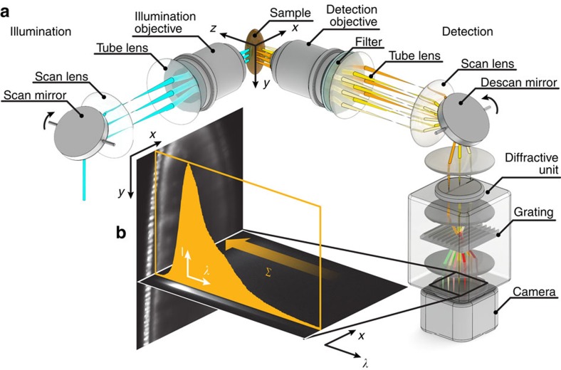
Figure 1
Hyperspectral SPIM setup and image formation.
( a ) Schematic of the setup. The light sheet is created by quickly scanning the illumination beam with a scan mirror. The sample is placed at the intersection of the focal planes of detection and ill...
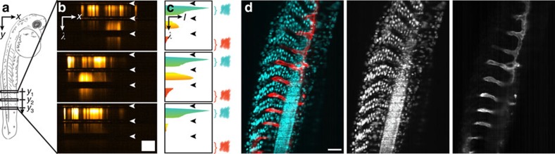
Figure 2
Image formation and virtual filtering.
( a ) Schematic drawing of a two days post fertilization zebrafish embryo imaged laterally. ( b ) Typical x , u03bb -data sets acquired along three different lines in a Tg(h2afva:h2afva-GFP,kdrl:Hsa.H...
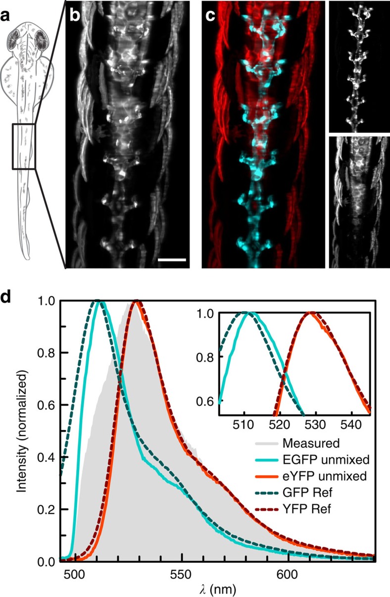
Figure 3
Linear unmixing of EGFP and eYFP.
( a ) Schematic drawing of a two days post fertilization zebrafish embryo imaged dorsally. ( b ) Integration of the reconstructed data set from a Tg(kdrl:EGFP,s1013t:Gal4,UAS:ChR2-eYFP) zebrafish alon...
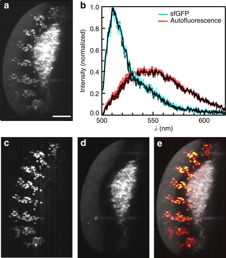
Figure 4
Unmixing of autofluorescence.
( a ) A u03bb -stack of 6u2009h post-laying Drosophila expressing sens -sfGFP was integrated between 500 and 570u2009nm to simulate imaging with a standard GFP bandpass filter. Strong autofluorescence...
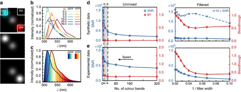
Figure 5
Optimal spectral sampling.
( a ) Synthetic data set consisting of spots exhibiting either EGFP (cyan) or eYFP (red) or the mean of both spectra (white). Spectral sampling, 0.5u2009nm per pixel. White frames, regions used to det...
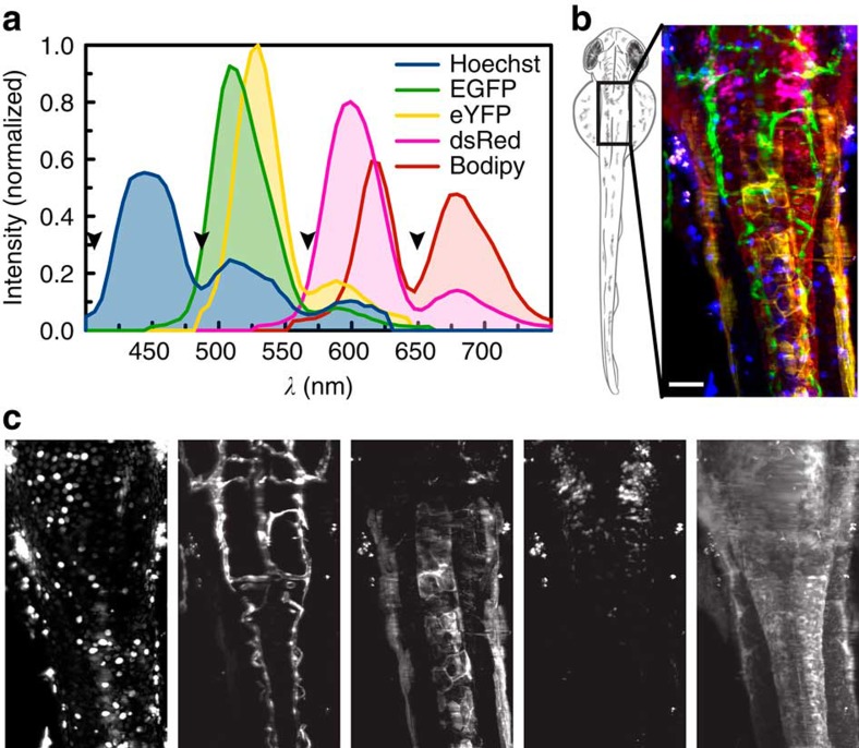
Figure 6
Linear unmixing of five fluorophores.
( a ) For imaging five colours, wild-type fish stained with Hoechst or Bodipy as well as fish expressing only EGFP, eYFP or dsRed were imaged to obtain reference spectra. Black arrowheads highlight re...
Figure images are served from the NIH/NLM PubMed Central Open Access Subset or Europe PMC; copyright remains with the publishers and authors.
💬 Discussion
0 commentsNo comments yet. Be the first to start a discussion!
Leave a Comment